Wide ReceiveR: Using PCA to group NFL Recievers Based Off Combine Measurements

How can we apply dimensionality reduction algorithms to NFL combine data in order to give us insight into the different types and archetypes of wide recievers drafted to the NFL?

What is the NFL Combine? Why is it important?

The NFL combine is an event that the National Football League (NFL) hosts every year to evaluate college athletes that will potentially be drafted by NFL teams. The combine typically occurs a few months before the NFL draft and the invited athletes undergo various athletic tests to determine how big, fast, and strong they are.

While players of all positions participate in the combine, it is especially important for wide receivers. Wide receivers are the players whose main job is to run down-field quickly and catch passes from the quarterback. Traits that are important for the success of wide receivers are primarily speed, explosiveness, and strength as they have to create space and separation from their defender. While some combine tests are infamously imprecise, for example, the NFL recently faced some push-back from their inclusion of an IQ test, these drills are quite applicable for wide receivers as how tall, fast, and strong they are is likely quite useful in projecting their performance in the league. Due to the applicability of combine drills to in-game performance, we chose to focus on this position in particular.

What are the athletic tests and what do they measure?

While a wide assortment of tests and measurements are taken at the combine, the 7 measurements and drills most wide receiver prospects participate in at the combine are described below.

Height: The height of a player is useful in determining a player’s catch radius or the amount of space around the player in which they can be expected to catch the ball. Taller players tend to have a larger catch radius as they can grab footballs that are thrown high in the air.

Weight: Helps us understand the body composition of the receiver. Is the receivers a thicker and more muscular player that can run through and break tackles?¹ Or is the player a thinner-limbed player who might struggle more with physicality and contact?

The lightest players are often wide receivers as speedy and elusive pass catchers can get by despite a lack of strength more easily than players at other positions. The lightest player in combine history is the receiver Brandon Banks, who weighted in at 149 pounds (the Football reference page generously rounds this up to 150 lbs).

40 yard-dash: The player runs 40 yards as fast as they can. This test is a good indicator of straight line speed which is very important for NFL pass catchers to create as much separation from their defenders as possible.

Bench: The bench press is a test that shows a player’s upper body strength. Players see how many times that can bench press a 225-pound weight.

The record holders for the bench press are mostly larger players who play other positions. However, the current Seattle Seahawks superstar wide receiver DK Metcalf, who has “internet-breaking” strength and size, caused quite a stir with his 27 repetition performance.

3-Cone Drill: This drill measures a players agility and ability to change directions quickly. Players seeing how quickly they can run back and forth between 3 cones.

Vertical: Players see how high they can jump. A high vertical is important in determining a players catch radius as it helps determine if they can catch balls thrown high in the air. Additionally, a higher vertical (as well as being taller in general) can help the wide receiver catch passes from above their defender.

Broad: Players see how far they can jump, this shows how explosive and athletic a player is.

Chris Conley, one of the wide receivers included in our PCA, has the third furthest broad jump measurement in NFL combine history at 11’7’’. Appropriately, our PCA grouped him into the “athletic paragon” archetype.

Where did we get our data? What data wrangling did we do? What is our question?

Our main question is: Can we determine the archetypes of different types of receivers in the NFL based off of combine data?

First, we scraped a majority of our data from NFL Savant, which gave us the data on NFL combine athletic testing results.

Show code

library(tidyverse)
library(rvest)
library(ggrepel)
library(nflfastR)
library(gsisdecoder)
library(plotly)
library(gt)
library(grid)
library(ggradar2)


#Storing url
url_12 <- "http://www.nflsavant.com/draft.php?ln=&fn=&college=&height=&hegt=%3E&weight=&wgt=%3E&arm_length=&argt=%3E&hand_size=&hagt=%3E&forty=&fgt=%3E&shuttle=&shgt=%3E&vertical=&vgt=%3E&bench=&bgt=%3E&cone=&cgt=%3E&p=WR&broad=&brgt=%3E&round=&rgt=%3E&year=2012&wonder=&wogt=%3E&submit=true#results"

url_13 <- "http://www.nflsavant.com/draft.php?ln=&fn=&college=&height=&hegt=%3E&weight=&wgt=%3E&arm_length=&argt=%3E&hand_size=&hagt=%3E&forty=&fgt=%3E&shuttle=&shgt=%3E&vertical=&vgt=%3E&bench=&bgt=%3E&cone=&cgt=%3E&p=WR&broad=&brgt=%3E&round=&rgt=%3E&year=2013&wonder=&wogt=%3E&submit=true#results"
  
url_14 <- "http://www.nflsavant.com/draft.php?ln=&fn=&college=&height=&hegt=%3E&weight=&wgt=%3E&arm_length=&argt=%3E&hand_size=&hagt=%3E&forty=&fgt=%3E&shuttle=&shgt=%3E&vertical=&vgt=%3E&bench=&bgt=%3E&cone=&cgt=%3E&p=WR&broad=&brgt=%3E&round=&rgt=%3E&year=2014&wonder=&wogt=%3E&submit=true#results"

url_15 <- "http://www.nflsavant.com/draft.php?ln=&fn=&college=&height=&hegt=%3E&weight=&wgt=%3E&arm_length=&argt=%3E&hand_size=&hagt=%3E&forty=&fgt=%3E&shuttle=&shgt=%3E&vertical=&vgt=%3E&bench=&bgt=%3E&cone=&cgt=%3E&p=WR&broad=&brgt=%3E&round=&rgt=%3E&year=2015&wonder=&wogt=%3E&submit=true#results"

total_12 <-  url_12 %>%
  read_html %>%
  html_nodes(xpath = " /html/body/div/div[10]/div[3]/table") %>%
  html_table( fill = TRUE )


total_13 <-  url_13 %>%
  read_html %>%
  html_nodes(xpath = " /html/body/div/div[10]/div[3]/table") %>%
  html_table( fill = TRUE )

total_14 <-  url_14 %>%
  read_html %>%
  html_nodes(xpath = " /html/body/div/div[10]/div[3]/table") %>%
  html_table( fill = TRUE )

total_15 <-  url_15 %>%
  read_html %>%
  html_nodes(xpath = " /html/body/div/div[10]/div[3]/table") %>%
  html_table( fill = TRUE )


nfl_combine_12<-total_12[[1]]

nfl_combine_13<-total_13[[1]]

nfl_combine_14<-total_14[[1]]

nfl_combine_15<-total_15[[1]]

After scraping these tables, we realized that a lot of these results came from “draft busts” or players who didn’t perform well in the NFL and were either did not make or did not last long on the roster of professional football teams. We wanted to clear up some of the clutter in our PCA and utilized Ben Baldwin’s NFL package to filter out players who didn’t have more than 50 catches in a season by their first 3 regular seasons, a reasonable bar for starting wide receivers.² This filter removes players whose contributions were not notable and leaves us with a list of receivers who are likely to be recognized by most NFL fans.

Show code

#Grabbing regular season data from 3 years post draft

games_2017 <- nflfastR::load_pbp(2017) %>% dplyr::filter(season_type == "REG")
games_2017 <- games_2017 %>%
  dplyr::filter(!is.na(xyac_mean_yardage))

#Filtering out non recievers (eg defensive players etc)

games_2017 <- games_2017 %>%
  dplyr::filter(!is.na(receiver_id))

#Counting the number of times they were credited with a catch


WR_2014<-games_2017 %>%
  count (receiver) %>%
  filter (n>50) %>%
  arrange (desc(n))
#Using their last name as a ID for later join


WR_2014 <-WR_2014 %>%
  mutate(last_name=str_split(WR_2014$receiver, "\\."))

WR_2014<-WR_2014 %>%
  mutate(last_name_final = last_name[1])
#Creating dataset of productive players

names_WR_2014 <- c()
for (i in 1:120) {
  names_WR_2014[i] <- WR_2014$last_name[[i]][2]
}

#Repeat process
games_2016 <- nflfastR::load_pbp(2016) %>% dplyr::filter(season_type == "REG")
games_2016 <- games_2016 %>%
  dplyr::filter(!is.na(xyac_mean_yardage))

games_2016 <- games_2016 %>%
  dplyr::filter(!is.na(receiver_id))


WR_2013<-games_2016 %>%
  count (receiver) %>%
  filter (n>50) %>%
  arrange (desc(n))


WR_2013 <-WR_2013 %>%
  mutate(last_name=str_split(WR_2013$receiver, "\\."))

WR_2013<-WR_2013 %>%
  mutate(last_name_final = last_name[1])

names_WR_2013 <- c()
for (i in 1:131) {
  names_WR_2013[i] <- WR_2013$last_name[[i]][2]
}

games_2015 <- nflfastR::load_pbp(2015) %>% dplyr::filter(season_type == "REG")
games_2015 <- games_2015 %>%
  dplyr::filter(!is.na(xyac_mean_yardage))

games_2015 <- games_2015 %>%
  dplyr::filter(!is.na(receiver_id))


WR_2012<-games_2015 %>%
  count (receiver) %>%
  filter (n>50) %>%
  arrange (desc(n))


WR_2012 <-WR_2012 %>%
  mutate(last_name=str_split(WR_2012$receiver, "\\."))

WR_2012<-WR_2012 %>%
  mutate(last_name_final = last_name[1])

names_WR_2012 <- c()
for (i in 1:125) {
  names_WR_2012[i] <- WR_2012$last_name[[i]][2]
}

games_2014 <- nflfastR::load_pbp(2014) %>% dplyr::filter(season_type == "REG")
games_2014 <- games_2014 %>%
  dplyr::filter(!is.na(xyac_mean_yardage))

games_2014 <- games_2014 %>%
  dplyr::filter(!is.na(receiver_id))


WR_2011<-games_2014 %>%
  count (receiver) %>%
  filter (n>50) %>%
  arrange (desc(n))


WR_2011 <-WR_2011 %>%
  mutate(last_name=str_split(WR_2011$receiver, "\\."))

WR_2011<-WR_2011 %>%
  mutate(last_name_final = last_name[1])

names_WR_2011 <- c()
for (i in 1:122) {
  names_WR_2011[i] <- WR_2011$last_name[[i]][2]
}


games_2013 <- nflfastR::load_pbp(2013) %>% dplyr::filter(season_type == "REG")
games_2013 <- games_2013 %>%
  dplyr::filter(!is.na(xyac_mean_yardage))

games_2013 <- games_2013 %>%
  dplyr::filter(!is.na(receiver_id))


WR_2010<-games_2013 %>%
  count (receiver) %>%
  filter (n>50) %>%
  arrange (desc(n))


WR_2010 <-WR_2010 %>%
  mutate(last_name=str_split(WR_2010$receiver, "\\."))

WR_2010<-WR_2010 %>%
  mutate(last_name_final = last_name[1])

names_WR_2010 <- c()
for (i in 1:133) {
  names_WR_2010[i] <- WR_2010$last_name[[i]][2]
}

games_2012 <- nflfastR::load_pbp(2012) %>% dplyr::filter(season_type == "REG")
games_2012 <- games_2012 %>%
  dplyr::filter(!is.na(xyac_mean_yardage))

games_2012 <- games_2012 %>%
  dplyr::filter(!is.na(receiver_id))

WR_2009<-games_2012 %>%
  count (receiver) %>%
  filter (n>50) %>%
  arrange (desc(n))

WR_2009 <-WR_2009 %>%
  mutate(last_name=str_split(WR_2009$receiver, "\\."))

WR_2009<-WR_2009 %>%
  mutate(last_name_final = last_name[1])

#Creating dataset of productive players
names_WR_2009 <- c()
for (i in 1:125) {
  names_WR_2009[i] <- WR_2009$last_name[[i]][2]
}


#2015 combine so 2018 catches

names_15 <- nfl_combine_15 %>%
  mutate (full_name = str_c(First, Last, sep = " ", collapse = NULL))


names_15_filtered <- names_15 %>%
  filter (Last %in% c(names_WR_2014,names_WR_2013,names_WR_2012))


#2014 combine so 2017 catches


names_14 <- nfl_combine_14 %>%
  mutate (full_name = str_c(First, Last, sep = " ", collapse = NULL))


names_14_filtered <- names_14 %>%
  filter (Last %in% c(names_WR_2013,names_WR_2012,names_WR_2011))



#2013 combine so 2016 catches


names_13 <- nfl_combine_13 %>%
  mutate (full_name = str_c(First, Last, sep = " ", collapse = NULL))


names_13_filtered <- names_13 %>%
  filter (Last %in% c(names_WR_2012,names_WR_2011,names_WR_2010))


#2012 combine so 2015 catches


names_12 <- nfl_combine_12 %>%
  mutate (full_name = str_c(First, Last, sep = " ", collapse = NULL))


names_12_filtered <- names_12 %>%
  filter (Last %in% c(names_WR_2011,names_WR_2010,names_WR_2009))

total_filtered <- rbind(names_12_filtered, names_13_filtered, names_14_filtered, names_15_filtered)

We then used the data to create a PCA algorithm that aimed to reduce the dimensionality of the combine data, which originally lives in the 7th dimension due to the 7 measurements we utilized. A PCA functions by taking data and finding the best combination of proportions of various variables to create divisions or sections of archetypes. This explanation might seem somewhat abstract and will hopefully be aided by looking at what our actual principal components represent, which will be done below. PCAs often require “domain knowledge” or specialized knowledge of the data in order to interpret. While we certainly do not claim to be NFL draft gurus, we were lucky that our principal components fell into three general groups of speed, athleticism, and strength–the three categories that your average NFL fan would probably come up with if asked to summarize the important traits of a wide receiver.

One point of note is that players who are worried about being penalized in the draft due to a certain weakness would sometimes skip certain drills or tests at the combine that emphasize their flaws. However, the PCA cannot easily process “NA”s. Hence, in order to approximate missing data resulting from skipped drills, we substituted in the value of the bottom 15th percentile as players would only skip the drills that they felt the least confident about.

Show code

#Some repeat last names

total_filtered <- total_filtered[-c(12, 1,2,75,5,30,55,81,82,83,59,34,15,61,88,22,37,39,95,96,97,23), ]

#Assigning 15th percentile scores to players who skipped a certain test
total_filtered[,8] <- ifelse(total_filtered[,8] == 0, quantile(total_filtered[,8], 0.85), total_filtered[,8])

total_filtered[,9] <- ifelse(total_filtered[,9] == 0, quantile(total_filtered[,9], 0.15), total_filtered[,9])


total_filtered[,10] <- ifelse(total_filtered[,10] == 0, quantile(total_filtered[,10], 0.85), total_filtered[,10])


 
for (i in 11:14 ){
  
 total_filtered[,i] <- ifelse(total_filtered[,i] == 0, quantile(total_filtered[,i], 0.15), total_filtered[,i])

}



PCA_final <- total_filtered %>%
  select(Height, Weight, "40YD", Bench, "3Cone", Vertical, Broad)

PCA_final<-scale(PCA_final)


pca <- prcomp(PCA_final)

d <- as.data.frame(pca$x)

pc1 <- pca$rotation[, 1]

pc2 <- pca$rotation[, 2]

pc3 <- pca$rotation[, 3]



total_names_filtered<- total_filtered %>%
  mutate (PC_one = d$PC1,
          PC_two = d$PC2,
          PC_three = d$PC3)

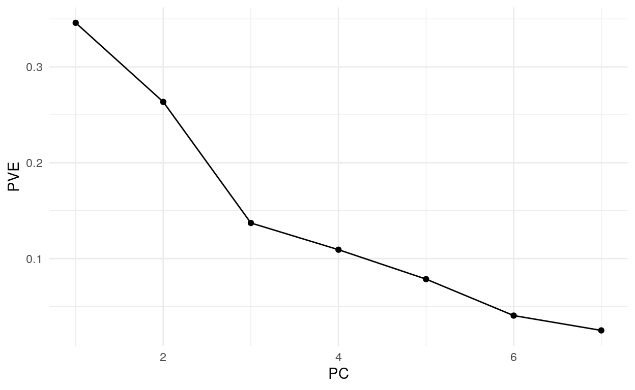
Additionally, we had to decide the number of principal components to use in our analysis. In order to visualize our data, we knew that we had to reduce dimensionality to either 2- or 3-dimensions. In order to determine how many components to use, we referred to our scree plot, which plots the amount of unexplained variability (PVE) as a function of the number of components. We wanted to minimize the unexplained variability while not including too many principal components. When looking at the plot, the lowest unexplained variability is with 7 principal components, which makes sense as we are no longer reducing dimensionality in that case. We saw a distinct “elbow” at PC=3 where including any more than 3 principal components does not increase the explained variability by too much. We ultimately went with 3 principal components which explains 86.3% of the variability in the data, not bad for a dataset that uses less than half the number of original variables! Choosing 3 principal components would also allow us to plot our data in a 3-dimensional plane, making for relatively easy visualization. The specific principal components are described below.

Show code

d1 <- tibble(PC = 1:7,
                PVE = pca$sdev^2 /
                  sum(pca$sdev^2))

ggplot(d1, aes(x = PC, y = PVE)) +
  geom_line() + 
  geom_point()+
  theme_minimal()

Examining the Principal Components

Here, domain knowledge comes into play as we have to interpret what these principal components are truly measuring and why certain variables are grouped together. Each variable’s weights in the respective principal components are shown in the table below and, underneath that, we attempt to explain what the principal component represents in terms of football.

Show code

pc1_gt <- as.data.frame(pc1)
pc2_gt <- as.data.frame(pc2)
pc3_gt <- as.data.frame(pc3)

pc1_gt <- pc1_gt %>%
  pivot_wider(names_from = pc1, values_from = pc1)

pc2_gt <- pc2_gt %>%
  pivot_wider(names_from = pc2, values_from = pc2)

pc3_gt <- pc3_gt %>%
  pivot_wider(names_from = pc3, values_from = pc3)

colnames(pc1_gt) <- c("Height", "Weight", "40YD", "Bench", "3Cone", "Vertical", "Broad")
colnames(pc2_gt) <- c("Height", "Weight", "40YD", "Bench", "3Cone", "Vertical", "Broad")
colnames(pc3_gt) <- c("Height", "Weight", "40YD", "Bench", "3Cone", "Vertical", "Broad")

pc12_gt <- full_join(pc1_gt, pc2_gt, by = NULL)

pca_gt <- full_join(pc12_gt, pc3_gt, by = NULL)

pca_gt <- bind_cols(pca_gt, pc_name = c('PC1', 'PC2', 'PC3'))

pca_gt <- pca_gt %>%
  relocate(pc_name, .before = Height)

pca_gt %>%
  gt() %>%
  cols_label("pc_name" = "PC Name",
            "Height" = "Height", 
            "Weight" = "Weight",
             "40YD" = "40 Yard Dash",
             "Bench" = "Bench Press",
            "3Cone" = "3 Cone Drill",
            "Vertical" = "Vertical Jump",
            "Broad" = "Broad Jump") %>%
  tab_header(title = "NFl Combine PCAs") %>%
  tab_spanner(label = "Athletic Tests",
          column = vars("Height",
                    "Weight",
                   "40YD",
                   "Bench",
                   "3Cone",
                   "Vertical",
                   "Broad")) %>%
  data_color(
columns = vars("Height",
                    "Weight",
                   "40YD",
                   "Bench",
                   "3Cone",
                   "Vertical",
                   "Broad"),
colors = as.character(paletteer::paletteer_d("ggsci::purple_material",
                                    n = 8)
)) 

NFl Combine PCAs
PC Name	Athletic Tests
	Height	Weight	40 Yard Dash	Bench Press	3 Cone Drill	Vertical Jump	Broad Jump
PC1	-0.4093328	-0.429923901	-0.4577419	-0.1765625	-0.39348067	0.36682709	0.3428134
PC2	0.4578382	0.456967427	-0.1391618	0.1793624	0.03086603	0.48915333	0.5383348
PC3	-0.1476090	-0.009999411	-0.1632238	0.9287666	-0.24615671	-0.04597659	-0.1617254

PC1

A player who scores highly on PC1 is short and light, but also fast and agile. Considering that height, weight, 40-yard dash, and 3 cone drill all have negative coefficients, heavier and slower players will be penalized (because a higher 40 yard or 3 cone time is slow, a negative coefficient actually rewards faster players). This player is typically relatively explosive with decent vertical and broad jumps but typically quite weak. On the interactive graph, this PC is the X axis and is called “Speed and Shiftiness”.

PC2

PC2 assigns the most significance to a player’s height, weight, as well as explosiveness (quantified through vertical and broad jump) as these have the highest coefficients. The relatively small or even nonexistent penalties for slow 40 yard dash and 3 cone drills means that high scorers on PC2 often have subpar speed but make up for it with above average size and impressive verticals and broad jumps. On the interactive graph we called this principal component “Explosiveness” and placed it on the Y axis.

Fascinatingly, this PC aligns most neatly with what is conventionally thought of as “athleticism”. One site used often by draft experts is “Relative Athleticism Score”, which essentially calculates a player’s percentile ranks for each of their combine measurements as compared to their position. The 5 wide receivers that scored the highest on PC2 scored an average relative athleticism score of 9.4/10. Pretty impressive when you considered that they are normalized against some of the best athletes in the country! It is interesting that relative athleticism seems to favor lateral explosiveness over speed or strength.

PC3

Interestingly, the vast majority of a player’s PC3 score comes from a single metric: bench press. The 0.92 coefficient for bench on PC3 is by far the highest value of any of our weights and thus PC3 is largely determined by a players strength. Interestingly, height and broad jump have moderate, negative coefficients, so the highest scorers are those that are short, not very explosive, but incredibly strong. On our interactive graph we placed this PC as the Z axis and called this PC “Strength”.

Creating and Exploring Archetypes

After going through what each of the principal components meant in the context of football, we created a set of archetypes based off of the values from each of the principal components. The archetypes are described below and examples are given before the data is visualized in 2 ways: an interactive 3D plot as well as radar plots.

Show code

#Preliminary grouping
total_names_filtered <- total_names_filtered %>%
  group_by(full_name) %>%
  mutate(group = if (PC_one <0 &  PC_two <0 &PC_three > 0  ){
    ("Immobile Bruiser")
  }
           else if (PC_one > 0 & PC_two > 0 & PC_three >0){
   ("Atheltic Paragon")
} else if (PC_one > 0 & PC_two <0 & PC_three <0){
   ("Undersized but Speedy")
} 
else if (PC_one > 0 & PC_two <0 & PC_three > 0){
   ("Undersized but Speedy")
} 
 else if (PC_one >0  & PC_two >0  & PC_three <0){
   ("Shifty and Elusive")
 } 
else if (PC_one <0 & PC_two >0 & PC_three <0 ){
   ("Explosive Playmaker")
} 
else if (PC_one <0 & PC_two >0 & PC_three >0 ){
   ("Explosive Playmaker")
 } 

else if ((PC_one <0 & PC_two <0 & PC_three <0)){
   ("Intelligent Route Runner")
} 
else {
  "Determine Later"
})

Athletic Paragon: This player is extremely fast (PC 1 < 0) ³, explosive (PC 2 > 0), and strong (PC 3 > 0). These players are all-around elite athletes and include some of the most electrifying athletes in the sport. Examples include Davante Adams and [Odell Beckham Jr](https://www.pro-football-reference.com/players/B/BeckOd00.htm.

Explosive Playmaker: This player is extremely explosive (PC 2 > 0) but quite slow (PC 1 >0). Considering that these players rely on out-leaping their defenders to catch passes that were placed high in the air, upper body strength is less important to these players and thus both stronger and weaker players will grouped together (PC 3 > or < 0). These players don’t necessarily always outrun their defenders but have a greater catch radius due to their ability to leap up and catch high paces placed over their defenders. Examples include Deandre Hopkins and Mike Evans.

Immobile Bruiser: This player is extremely strong (PC 3 > 0), but very slow (PC 1 < 0) and un-explosive (PC 2 > 0). These players are hard to take down or tackle and can make catches by outmuscling defenders. Examples include Jarvis Landry and Nelson Agholor.

Intelligent Route Runner: This player is slow (PC 1 > 0), weak (PC 3 < 0), and un-explosive (PC 2 < 0), in other words, below average in all categories. As a result, the only way they could’ve gotten drafted is due to their on-field intelligence and game sense. These players’ feel for the game and footwork allows them to get open. Examples include one of the authors’ favorite pass catchers: Keenan Allen⁴

Shifty and Elusive: This player is extremely fast (PC 1 < 0) and explosive (PC 2 > 0) but the weakest of all archetypes (PC 3 < 0). Examples include Marqise Lee and Alshon Jeffery⁵.

Undersized but Speedy: This player is defined by their speed (PC 1 < 0) but lacks in explosiveness and size (PC 2 < 0). Because these players are reliant upon outrunning their defenders rather than muscling through them, strength was not considered (both PC 3 > 0 and <0 were included). A great example is the other author’s favorite receiver-the 5’9, 166 pound Marquise “Hollywood” Brown⁶.

Interactive 3D Plot

Below we see the first visualization of our principal components and archetypes in an interactive 3D plot. To remove an archetype from the 3D plot, left click the archetype label in the legend once. To focus on one archetype and filter out the rest, left click the label twice. Player name and details can be found by hovering over the points. While the basics of each archetype have already been described, it is quite interesting to see where each player falls relative to others in their archetype. For example, even compared to other “athletic paragons”, Chris Conley stands out for his combination of explosiveness, speed, and strength⁷.

Show code

total_names_filtered <- total_names_filtered %>%
  mutate (archetype = as.factor (group))



fig <- plot_ly(total_names_filtered, x = ~PC_one, y = ~PC_two, z = ~PC_three,  color = ~archetype,colors = c('#BF382A', '#0C4B8E', "#FF7F50","#6495ED", "#CCCCFF","#40E0D0", "#9FE2BF"),
               text = ~full_name,
    hovertemplate = paste(
      "<b>%{text}</b><br>",
      "Speed: %{x}<br>",
      "Explosiveness: %{y}<br>",
      "Strength: %{z}<br>"))


fig <- fig %>% add_markers()
fig <- fig %>% layout(scene = list(xaxis = list(title = 'Speed and Shiftiness'),
                     yaxis = list(title = 'Explosiveness'),
                     zaxis = list(title = 'Strength')))





fig

Radar Plots

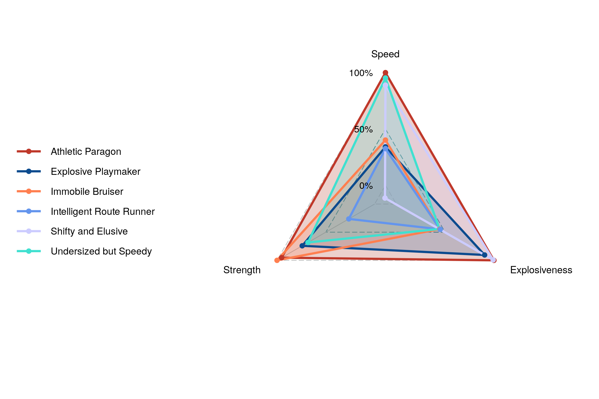
If 3D plots are not your thing, fear not! We also plotted out our PCA results on radar charts⁸, which provides a 2D visualization of the same data.

Players were grouped by archetypes and then had their principal component values averaged. The position of the vertices of the triangle on each gridline represents the relative value of each principal component, the closer to the edge of the shaded gray triangle, the better that archetype scored on that particular trait. The percentages were derived by taking that archetype’s value and dividing it by the value of the highest archetype. Unsurprisingly, the “athletic paragons” had the highest values for principal components 1 and 2 (speed and athleticism) and was only a little behind the “immobile bruisers” for strength; hence, they have the largest triangle as they represent the 100% value for 2 of the 3 principal components.

The shape of the triangle also helps show the relative balance between these traits. Some archetypes end up with near equilateral triangles, these archetypes are either impressive in all categories, such as the athletic paragons, or below average in every realm, as is the case with the intelligent route runners. On the other hand, archetypes such as immobile bruisers have isolateral distributions as they perform well on strength measures but poorly on the other two categories.

Show code

summary<- total_names_filtered %>%
  group_by (archetype) %>%
  summarize (avg_one = mean (PC_one),
             avg_two = mean (PC_two),
             avg_three = mean (PC_three))


summary <- summary[,2:4]
summary <- as.data.frame(summary)

rownames(summary) <- c( "Athletic Paragon", "Undersized but Speedy", "Immobile Bruiser", "Explosive Playmaker", "Shifty and Elusive", "Intelligent Route Runner")

spider_df <- summary %>% rownames_to_column("group")

colnames(spider_df) <- c("group", "Speed", "Explosiveness", "Strength")


spider_plot<-ggradar2(spider_df, 
        group.colours  =c('#BF382A', '#0C4B8E', "#FF7F50","#6495ED", "#CCCCFF","#40E0D0", "#9FE2BF"), 
        group.fill.colours = c('#BF382A', '#0C4B8E', "#FF7F50","#6495ED", "#CCCCFF","#40E0D0", "#9FE2BF"), 
  grid.min = -5,  grid.max = 2.5, , fullscore = c(1.4426516,1.429569,0.59650617),radarshape  = "sharp")

spider_plot

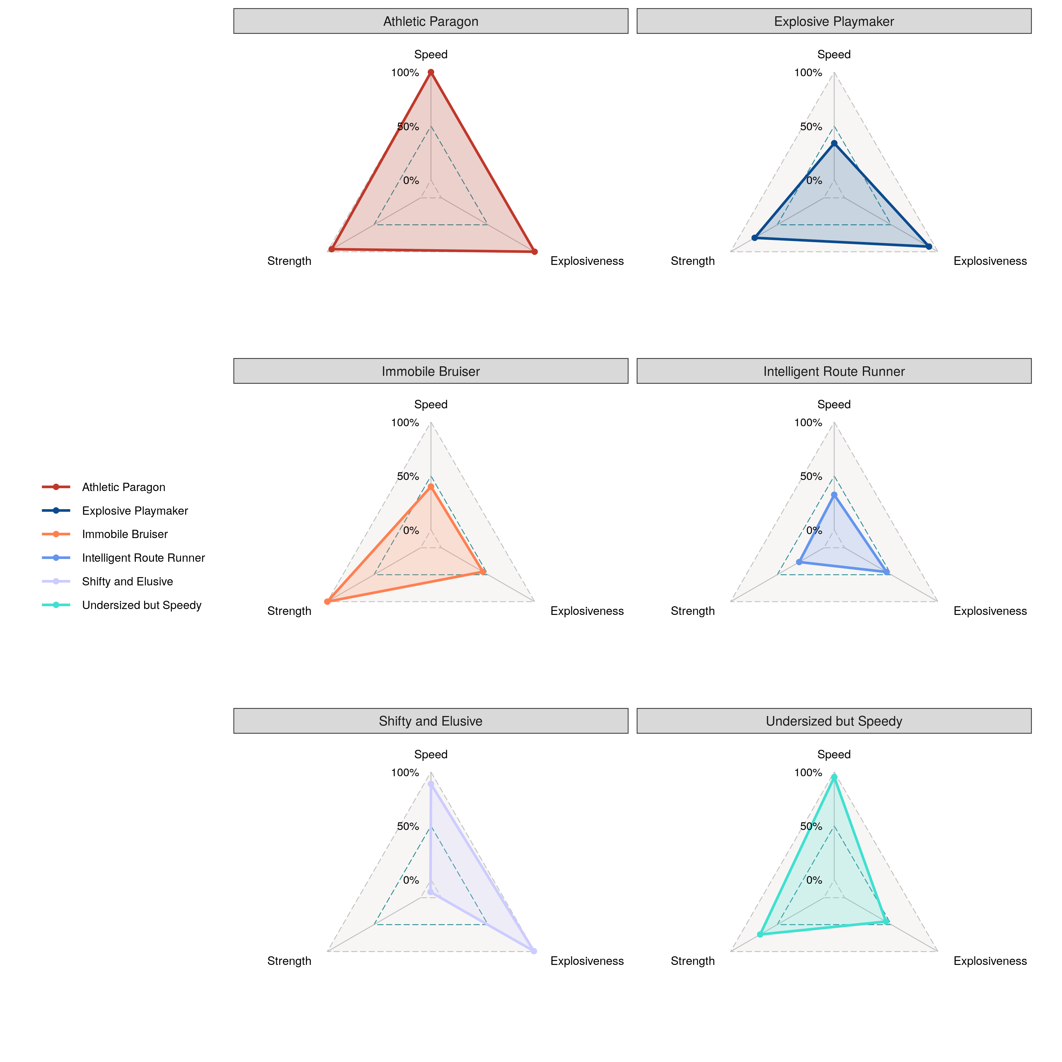
If the overlaid radar plot is too hectic for you, don’t worry! It was a bit busy for us as well, which is why we split the 6 archetypes up below. The differences in shape and size of the polygons between archetypes are now much more apparent. Trends such as the extreme lack of upper body strength among players falling into the “shifty and elusive” category⁹ are highlighted.

Show code

spider_plot + facet_wrap(. ~ group, nrow = 3)

Conclusion

Our PCA algorithm created 3 principal components that line up quite neatly with the traits that are important for pass catchers: speed, explosiveness, and strength. From this, we were able to create 6 groupings of players: Athletic Paragon, Undersized but Speedy, Immobile Bruiser, Explosive Playmaker, Shifty and Elusive, and Intelligent Route Runner. Our PCA explains 86.3% of the variability in our combine data, thus preventing too much loss of information while allowing for easy visualization and grouping. After looking at our findings, it becomes clear that to be drafted as a receiver in the NFL, one must measure incredibly well in at least one, if not all, of the categories of speed, strength, size, and explosiveness. While our PCs measure the physical measurable of players who are drafted, one shortcoming is that there is no way to numerically quantify important immeasurable qualities like smart route-running, football intellect, and work-ethic, all of which are traits that lead to a player being drafted and having successful NFL careers. Nonetheless, we hope that this post was both entertaining and informative in understanding the dimensions and archetypes of pass catchers in the NFL.

---

1. Breaking a tackle describes a player’s ability to stay upright after getting tackled, a desirable trait as the play is live as long as the player does not fall to the ground.↩︎

2. The first three seasons of a player’s career were considered due to the amount of late bloomers who really started making a contribution in year 2 or 3. Going from college to the NFL is difficult and we wanted to cast a wider net.↩︎

3. Remember that higher times actually mean slower runners, thus, lower scores on PC one actually represent faster players.↩︎

4. Appropriately, one article claims that “Allen’s top attribute has always been his mind” and adds that “Allen wins with his mind as much as his body”. These seem like backhanded compliments but running intelligent routes is a trait that pays well.↩︎

5. Neither player attempted the bench press at the combine, suggesting their relative lack of upper body strength.↩︎

6. Brown’s nickname among friends is “Jet” due to his blazing speed↩︎

7. One article crowns him as the most athletic receiver in his draft and called him the “full package”. The article also notes his 100th percentile broad and long jump measurements, truly a paragon of athleticism.↩︎

8. These charts are also called spider charts as, with increasing number of dimensions, they begin to look like spider webs. However, given that we only have 3 dimensions, spider webs that resemble our plots would be quite sad indeed.↩︎

9. You don’t have to fight through tackles if you can’t be caught I suppose.↩︎