Data Preperation
The dataset used in this blog comes from Kaggle. It contains detaied information of all Airbnb accommodations in United States up until Oct, 2020.
Show code
#Load necessary packages
library(knitr)
library(tidyverse)
library(ggplot2)
library(readr)
library(here)
library(ggmap)
library(leaflet)
library(tidycensus)
library(lubridate)
library(httr)
library(glue)
library(stringr)
library(tidytext)
library(wordcloud)

#Import Data
airbnb <- read_csv(here("_posts/2021-05-11-under-the-roof-a-general-view-of-airbnbs-in-the-us/data/AB_US_2020.csv"))

#filter out unconventional observations
airbnb <- airbnb %>%
  filter(city != "Hawaii", price >= 5, number_of_reviews != 0)
What’s going on across the country
Where are they located?
Show code
states <- map_data("state")
ggplot(data = states, mapping = aes(x = long, y = lat,
group = group)) +
geom_polygon(fill = "#2a7ac9", color = "white") +
coord_fixed(1.3) +
geom_point(data = airbnb, aes(longitude, latitude),
color = "#bd3333", alpha = 0.8,
inherit.aes = FALSE) +
theme_void() +
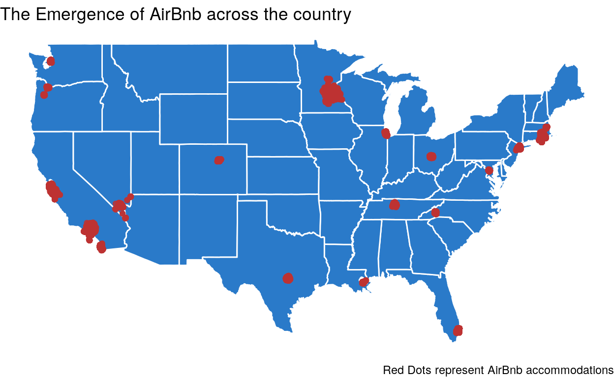
labs(title = "The Emergence of AirBnb across the country", caption = "Red Dots represent AirBnb accommodations")
Show code
counts_summary <- airbnb %>%
  group_by(city) %>%
  summarise(number_of_accommodations = n(),
            number_of_reviews = sum(number_of_reviews)) %>%
  arrange(desc(number_of_accommodations))
options(knitr.table.format = "html")
kable(counts_summary, digits = 2,
      caption = "Summary the number of accommodations across cities")
| city | number_of_accommodations | number_of_reviews |
|---|---|---|
| New York City | 35119 | 1032236 |
| Los Angeles | 24398 | 1113802 |
| San Diego | 10318 | 486335 |
| Broward County | 8336 | 233676 |
| Austin | 7660 | 317650 |
| Clark County | 6208 | 247679 |
| San Clara Country | 5795 | 212513 |
| Seattle | 5701 | 366233 |
| New Orleans | 5657 | 329407 |
| Washington D.C. | 5546 | 287084 |
| San Francisco | 5469 | 319331 |
| Nashville | 5333 | 335559 |
| Chicago | 5265 | 273496 |
| Twin Cities MSA | 4037 | 145779 |
| Portland | 3799 | 345936 |
| Denver | 3586 | 209019 |
| Rhode Island | 3125 | 112455 |
| Oakland | 2607 | 110627 |
| Boston | 2467 | 126851 |
| San Mateo County | 2435 | 137984 |
| Jersey City | 1966 | 70037 |
| Asheville | 1943 | 161983 |
| Santa Cruz County | 1436 | 101355 |
| Columbus | 1251 | 65191 |
| Cambridge | 833 | 48969 |
| Salem | 152 | 9109 |
| Pacific Grove | 145 | 13437 |
A high density of accommodations located long the west and east coast, mostly in those well-known tourist cities like New York and LA. Until now, New York City has the greatest number of 35,119 accommodations, and its total number of reviews is already over 1 million(See Table 1).
Average Price Ranking for Cities
Show code
we <- airbnb %>%
mutate(we = case_when(longitude > -98.35 ~ "east",
longitude <= -98.35 ~ "west"))
avg_city_price <- we %>%
select(city, price, we) %>%
group_by(city) %>%
mutate(average_price = mean(price)) %>%
select(city, average_price, we) %>%
distinct()
avg_city_price <- avg_city_price[order(avg_city_price$average_price), ]
avg_city_price$city <- factor(avg_city_price$city, levels = unique(avg_city_price$city))
price_by_city <- ggplot(avg_city_price, aes(x = city, y = average_price)) +
geom_bar(stat = "identity", aes(fill = we)) +
scale_fill_manual(name="East VS. West",
labels = c("Eastern area", "Western area"),
values = c("west"="#81bcf7", "east"="#2774c2")) +
coord_flip() +
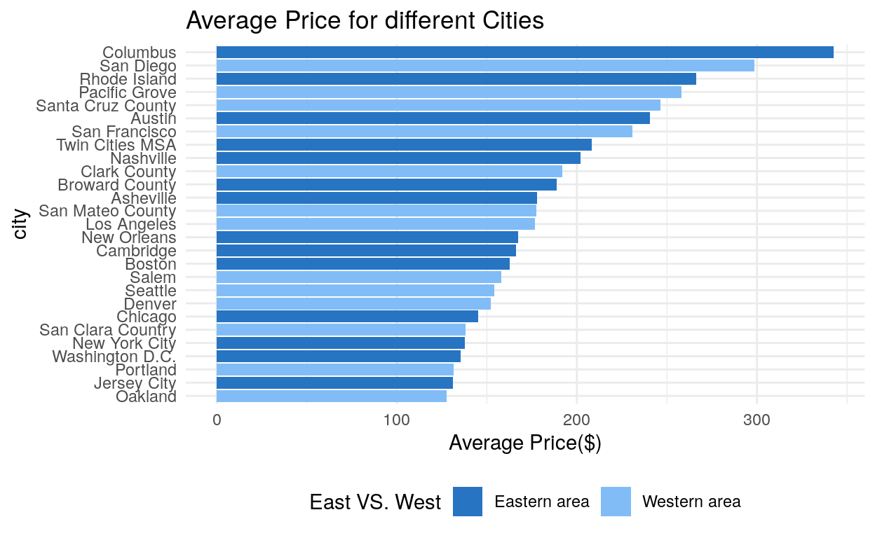
labs(title = "Average Price for different Cities", y = "Average Price($)") +
theme_minimal() +
theme(legend.position = "bottom")
price_by_city
Take a close look at Partland
Show code
#Make a new dataset for Portland
portland <- airbnb %>%
filter(city == "Portland")
#Make a wordcloud for the names of AirBnb
pal <- paletteer::paletteer_d("ggsci::teal_material",
n = 10)
portland %>%
unnest_tokens(output = word, input = name,
token = "words") %>%
anti_join(stop_words, by = "word") %>%
count(word, sort = TRUE) %>%
mutate(word = fct_reorder(word, n)) %>%
slice_max(n, n = 60) %>%
with(wordcloud(word, n, colors = pal,
random.order = FALSE,
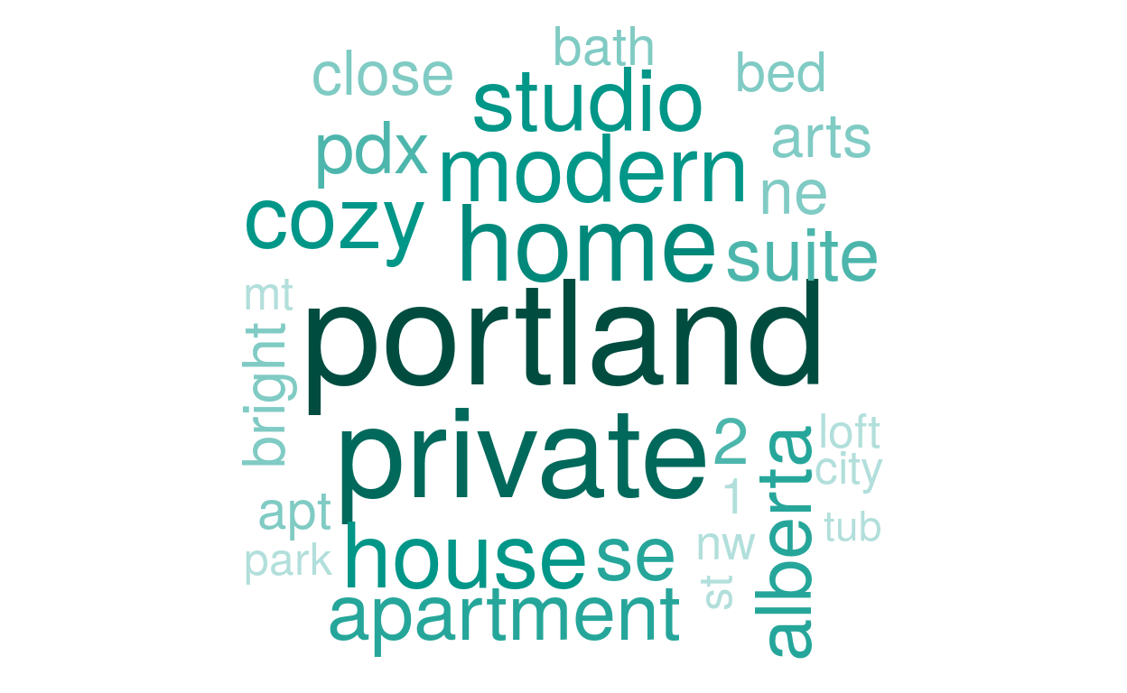
scale = c(5, 1)))
Make it interactive!
Show code
#Makes the icon and popup for the map
house  <- makeIcon(
  iconUrl = "https://openclipart.org/image/800px/177826",
  iconWidth = 25, iconHeight = 40)

pop_content <- paste("<b>", portland$name,
                 "</b></br>", "Type:",
                 portland$room_type,
                 "</b></br>", "Price: $",
                 portland$price, "/night",
                 "</b></br>", "Number of Reviews:",
                 portland$number_of_reviews)

#Create interactive map
leaflet() %>%
  addTiles() %>%
  addMarkers(lng = ~longitude, lat = ~latitude,
             data = portland, clusterOptions = markerClusterOptions(),
             popup = pop_content, icon = house)
Zoom in and out to get a sense of how the accommodations are distributed in Portland, and click on the markers to get detailed information of each accommodation.
How’s the market price in Portland
Show code
#price distribution
ggplot(portland, aes(x = price)) +
geom_histogram(bins = 40, fill = "#3576cc", color = "white", alpha = 0.9) +
xlim(0, 500) +
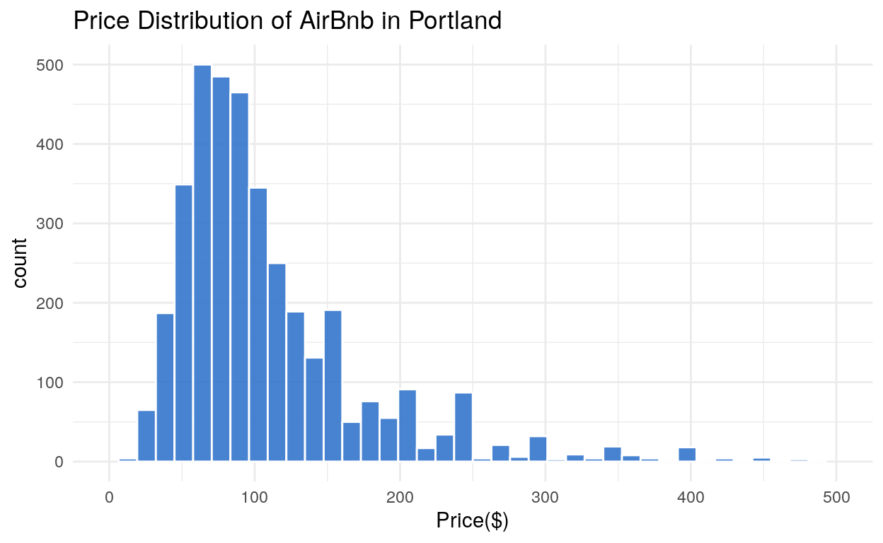
labs(title = "Price Distribution of AirBnb in Portland", x = "Price($)") +
theme_minimal()
Show code
| Mean | Median | Min | Max | StandardDev |
|---|---|---|---|---|
| 131.4 | 90 | 10 | 8400 | 247.47 |
While the average price AirBnb accommodations in Portland has a low ranking among all cities, it still has a medium of $90/night. The average rental price in Portland is approximately $1,509/month. The AirBnb is roughly three times expensive than long-term normal rent.
What makes it so pricy?
Even though the dataset doesn’t contain social factors, columns like “room_type” and “minimum_night” specify important features for every accommodations.
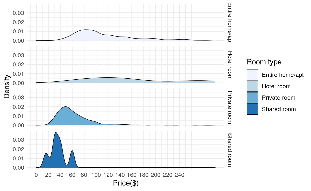
- Room Type
Show code
ggplot(portland, aes(price, fill = room_type)) +
  geom_density(position = "stack", size = 0.3)+
  facet_grid(room_type ~.)+
  scale_fill_brewer(palette = 1)+
  scale_x_continuous(limits = c(0,300), breaks = seq(0,250,20))+
  labs(x = "Price($)", y = "Density", fill = "Room type")+
  theme_minimal()
Show code
| room_type | median_price | mean_price | n |
|---|---|---|---|
| Hotel room | 145 | 191.24 | 33 |
| Entire home/apt | 100 | 143.47 | 2898 |
| Private room | 55 | 86.65 | 848 |
| Shared room | 38 | 180.75 | 20 |
The density graphs of the four room types show very distinct distributions. Among four different types, shared room is the least common type, and has the lowest price distribution mostly falls below $80. The most expensive prices are for hotel rooms. The distribution cover a wide range a prices with a median of $145.
- Locations
Show code
#Divide price into three categories
portland_price <- portland %>%
  mutate(price_cat = case_when(price <= 40 ~ "Cheap",
                               price > 40 & price <= 250 ~ "Medium",
                               price > 250 ~ "Expensive"))

#Layers by price categories
cheap <- portland_price %>%
  filter(price_cat == "Cheap")
medium <- portland_price %>%
  filter(price_cat == "Medium")
expensive <- portland_price %>%
  filter(price_cat == "Expensive")

leaflet() %>%
  addTiles() %>%
  addCircleMarkers(lng = ~longitude, lat = ~latitude,
                   data = cheap, color = "#87e3ff", radius = 6,
                   stroke = FALSE, fillOpacity = 0.8, group = "Cheap") %>%
  addCircleMarkers(lng = ~longitude, lat = ~latitude,
                   data = medium,  color = "#07b0e3", radius = 6,
                   stroke = FALSE, fillOpacity = 0.8, group = "Medium") %>%
  addCircleMarkers(lng = ~longitude, lat = ~latitude,
                   data = expensive,  color = "#0d6fa1", radius = 6,
                   stroke = FALSE, fillOpacity = 0.8, group = "Expensive") %>%
  addLayersControl(overlayGroups = c("Cheap", "Medium", "Expensive"),
                   options = layersControlOptions(collapsed = FALSE))
How custermers react to the prices
To examine how sensitive customers are to prices, assume that the number of reviews is a good indicator of how popular the accommodation is.
Show code
portland_updated <- portland %>%
  filter(price <= 1500)

ggplot(portland_updated, aes(x = price, y = number_of_reviews)) +
  geom_point(alpha = 0.6, color = "#2a7ac9") +
  stat_smooth(fill = "#db796e", color = "#b53324", size = 0.8) +
  theme_minimal() +
  labs(title = "How does price affect Popularity", x = "Price($)", y = "Popularity")
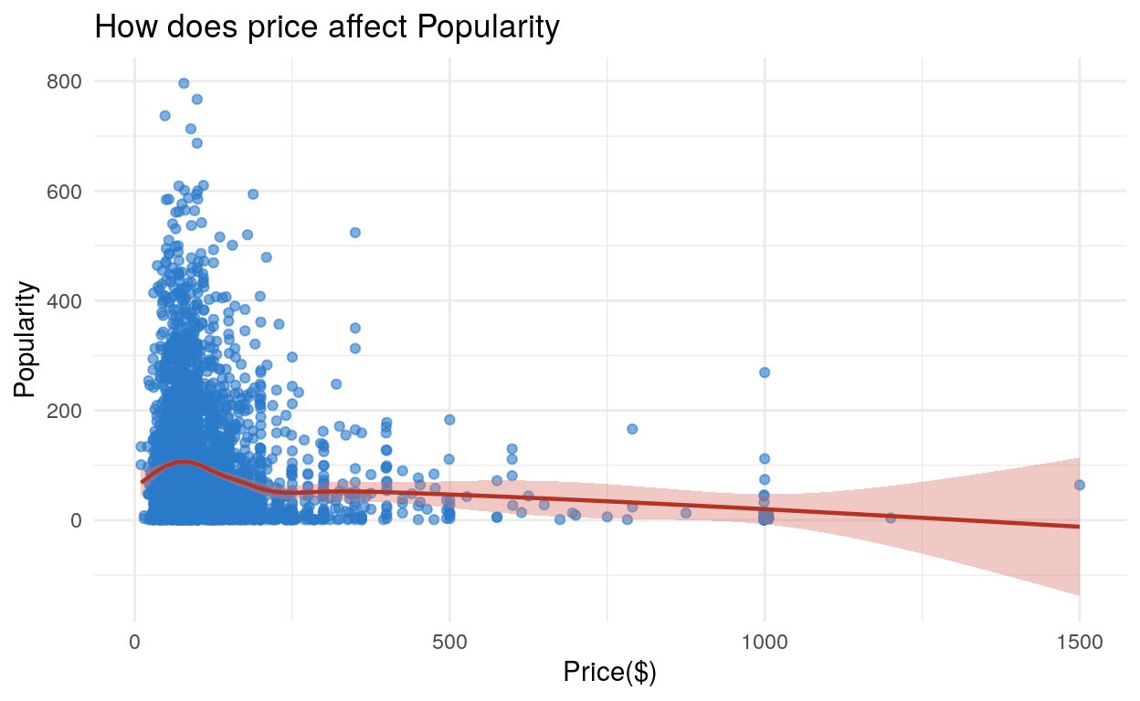
The graph above shows a reasonable tendency of change, the turning point of the regression line be around $80. Below this point, the popularity increases as the price increases; people seems to be careful with those extreme cheap accommodations. And above the turning point the popularity goes down as price increases, for these accommodations are less affordable.
Conclusion
This blog mainly looks a the physical factors of Airbnb accommodations and how they interact with each other. Considering that pricing and locations of accommodations are also heavily rely on the social surroundings, it would also be interesting if we combine the dataset with some local neighborhood statistics.