The differences between positive reviews are pretty clear—5 stars means a product is perfect and 4 stars means a product has a minor flaw. But what differentiates 1- and 2-star reviews (which are far more entertaining), in terms of their topics? To explore this question, we decided to focus on reviews for physical books because 1) the content of books is extremely diverse and 2) such books reviews might refer to either ‘structure’ (book condition), ‘function’ (book content) or both. To potentially capture a split between reviews about content and reviews about condition in our analysis, we attempted to only include reviews for paperback and hardcover editions of books.
We used topic modeling to try to identify distinct topics across reviews. Topic modeling is a method for analyzing text that assumes that words can have different meanings depending on their context. Unlike other forms of text analysis, topic models allow for each document of text to be assigned to multiple topics, depending on the number of topics the user specifies. Importantly, topic models do not explicitly identify and label topics, but learn topic groupings in an unsupervised manner; the user must subjectively infer the topic based on the model’s grouping. For instance, we might infer that the grouping of “petunia,” “daisy,” and “lily” refers to flowers.
We used Latent Dirichlet Allocation (LDA), the most common algorithm for topic modeling, in our analysis. LDA has two principles: 1) Every document is a mixture of topics and 2) Every topic is a mixture of words. LDA requires the user to specify the number of topics, k, for the model to identify. Each word in the corpus (all the texts) is then randomly assigned to one of the k topics. The topic assignments for each word are updated based on word frequencies and co-occurrences of words, so that the model (hopefully) creates more accurate groupings of words.
Nearly all of the code used in this post was adapted (with thanks!) from the following sources:
Scraping Amazon Reviews: Scraping Amazon Reviews in R
Preprocessing: A gentle introduction to text mining using R
Topic Modeling: A gentle introduction to topic modeling using R
Scraping from Amazon
In order to collect our data, we scraped the Amazon website for one- and two-star reviews of fiction books with a high number of reviews. For children’s books, the inclusion criteria was 20,000 reviews; for adult books, the minimum number of reviews was 30,000. We chose to use the number of reviews because it was a more stable measure of popularity than whether a book was on the bestsellers list, which updates frequently. Furthermore, we figured that books that have a high number of reviews could be more controversial, and hence have more negative reviews.
Below is a table showing the books we used in our the analysis.
Show code
book <- read_csv("data/Book1.csv")
book %>%
  dplyr::group_by(type) %>%
  arrange(`total reviews`) %>%
  gt() %>%
  cols_hide("ASIN") %>%
  cols_label(`book title` = "Title",
             `total reviews` = "Total reviews",
             `one-star review` = "1-star reviews",
             `two-star review` = "2-star reviews") %>%
  tab_header(title = "Fiction books used in our analysis") %>%
  tab_options(column_labels.font.weight = "bold",
              column_labels.font.size = "17px",
              column_labels.background.color = "midnightblue",
              row_group.background.color = "skyblue",
              heading.title.font.size = "25px",
              row_group.text_transform = "capitalize")
| Fiction books used in our analysis | |||
|---|---|---|---|
| Title | Total reviews | 1-star reviews | 2-star reviews |
| children | |||
| Harry Potter and the Half-Blood Prince | 22786 | 170 | 180 |
| Chicka Chicka Boom Boom | 22892 | 40 | 50 |
| Harry Potter and the Order of the Phoenix | 25465 | 150 | 170 |
| The Book Thief | 28709 | 360 | 340 |
| If animals kissed good night | 45020 | 150 | 60 |
| The Wonky Donkey | 55784 | 490 | 100 |
| adult | |||
| Ready Player One | 36666 | 560 | 460 |
| 1984 | 43120 | 270 | 220 |
| All the Light We Cannot See | 46294 | 580 | 750 |
| The Alchemist | 52556 | 410 | 260 |
| The Nightingale | 65062 | 520 | 350 |
| Where the Crawdads Sing | 128950 | 820 | 690 |
To scrape the data, we used the functions in the package rvest to create another function that automatically scrapes the title and text of each 1-star or 2-star review. To use the function, we need to put in a page range for the review, and the ASIN number to identify the book.
Below is the code to scrape one of the books.
Show code
# Setting up
# For one-star reviews
scrape_amazon1 <- function(ASIN, page_num){
  url_reviews <- paste0("https://www.amazon.com/product-reviews/",ASIN,"/?pageNumber=",page_num,"&filterByStar=one_star")

  doc <- read_html(url_reviews)

  doc %>%
    html_nodes("[class='a-size-base a-link-normal review-title a-color-base review-title-content a-text-bold']") %>%
    html_text() -> review_title

  doc %>%
    html_nodes("[class='a-size-base review-text review-text-content']") %>%
    html_text() -> review_text

  doc %>%
    html_nodes("[data-hook='review-star-rating']") %>%
    html_text() -> review_star

  tibble(review_title,
         review_text,
         review_star,
         page = page_num) %>% return()
}
# Children's book #5: Harry Potter and the Order of the Phoenix (5) (25,465)
ASIN <- "0439358078"
page_range <- 1:15
match_key <- tibble(n = page_range,
                    key = sample(page_range,length(page_range)))
lapply(page_range, function(i){

  j <- match_key[match_key$n==i,]$key

  scrape_amazon1(ASIN = ASIN, page_num = j)
}) -> output_list

data_onestar_children5 <- output_list[[1]]

for (i in 2:15) {
  data_onestar_children5 <- data_onestar_children5 %>%
    bind_rows(output_list[[i]])
}

# two-star review (similar function as scrape_amazon1)
ASIN <- "0439358078"
page_range <- 1:17
match_key <- tibble(n = page_range,
                    key = sample(page_range,length(page_range)))
lapply(page_range, function(i){

  j <- match_key[match_key$n==i,]$key

  scrape_amazon2(ASIN = ASIN, page_num = j)
}) -> output_list

data_twostar_children4 <- output_list[[1]]

for (i in 2:17) {
  data_twostar_children4 <- data_twostar_children4 %>%
    bind_rows(output_list[[i]])
}

# Combing one-star and two-star reviews:
children5 <- data_onestar_children5

write_csv(children5, "children5.csv")
Show code
# Loading the data
adult1 <- read_csv("data/adult1.csv")
adult2 <- read_csv("data/adult2.csv")
adult3 <- read_csv("data/adult3.csv")
adult4 <- read_csv("data/adult4.csv")
adult5 <- read_csv("data/adult5.csv")
adult6 <- read_csv("data/adult6.csv")

children1 <- read_csv("data/children1.csv")
children2 <- read_csv("data/children2.csv")
children3 <- read_csv("data/children3.csv")
children4 <- read_csv("data/children4.csv")
children5 <- read_csv("data/children5.csv")
children6 <- read_csv("data/children6.csv")

four_combinations_x <- read_csv("data/four_combinations_x.csv")
Review-level analysis
We initially labeled each book with a document ID, resulting in 12 documents (one for each book).
Show code
# expanding our data:
adult_1test <- adult1 %>%
  mutate(doc_id = 1,
         book_title = "The Alchemist")

adult_2test <- adult2 %>%
  mutate(doc_id = 2,
         book_title = "1984")

adult_3test <- adult3 %>%
  mutate(doc_id=3,
         book_title="Where the Crawdads Sing")

adult_4test <- adult4 %>%
  mutate(doc_id=4,
         book_title="Ready Player One")

adult_5test <- adult5 %>%
  mutate(doc_id=5,
         book_title="The Nightingale")

adult_6test <- adult6 %>%
  mutate(doc_id=6,
         book_title="All the Light We Cannot See")

children_1test <- children1 %>%
  mutate(doc_id = 7,
         book_title = "If Animals Kissed Good Night")

children_2test <- children2 %>%
  mutate(doc_id = 8,
         book_title = "Chicka Chicka Boom Boom")

children_3test <- children3 %>%
  mutate(doc_id = 9,
         book_title = "The Book Thief")

children_4test <- children4 %>%
  mutate(doc_id = 10,
         book_title = "Harry Potter and the Half-Blood Prince")

children_5test <- children5 %>%
  mutate(doc_id = 11,
         book_title = "Harry Potter and the Order of the Phoenix")

children_6test <- children6 %>%
  mutate(doc_id = 12,
         book_title = "The Wonky Donkey")

full_data <- adult_1test %>%
  rbind(adult_2test, adult_3test,
        adult_4test, adult_5test,
        adult_6test, children_1test,
        children_2test, children_3test,
        children_4test, children_5test,
        children_6test) %>%
  rename(text = review_text)
For our analysis, we decided to redefine the documents in terms of categories of reviews: 1-star reviews of children’s books, 2-star reviews of children’s books, 1-star reviews of adult books, and 2-star reviews of adult books. By creating the documents in this way, we would be able to compare between age level (children vs. adult) and number of stars (1 or 2). These divisions were chosen because the number of stars (1 or 2) pertained to our primary research question, while adult and children’s books were thought to be useful delineations because the content of adult fiction books are generally more complex.
Show code
#trimming white space
full_data$text <- full_data$text%>%
  trimws(which = "both", whitespace = "[ \t\r\n]")


#Filtering adult/child 1-star/2-star
adult_1star <- full_data %>%
  filter(review_star == "1.0 out of 5 stars",
         doc_id >= 1 & doc_id <= 6) %>%
  mutate(doc_id = 1)%>%
  select(text)
adult_2star <- full_data %>%
  filter(review_star == "2.0 out of 5 stars",
         doc_id >= 1 & doc_id <= 6) %>%
  mutate(doc_id = 2)%>%
  select(text)
children_1star <- full_data %>%
  filter(review_star == "1.0 out of 5 stars",
         doc_id >= 7 & doc_id <= 12) %>%
  mutate(doc_id = 3)%>%
  select(text)
children_2star <- full_data %>%
  filter(review_star == "2.0 out of 5 stars",
         doc_id >= 7 & doc_id <= 12) %>%
  mutate(doc_id = 4)%>%
  select(text)

adult_1star_x <- paste(adult_1star[,1], collapse = " ")

adult_1star_x <-adult_1star_x %>%
  as.data.frame() %>%
  mutate(doc_id = 1) %>%
  rename(text = ".")

adult_2star_x <- paste(adult_2star[,1], collapse = " ") %>%
  as.data.frame() %>%
  mutate(doc_id = 2) %>%
  rename(text = ".")

children_1star_x <- paste(children_1star[,1], collapse = " ") %>%
  as.data.frame() %>%
  mutate(doc_id = 3) %>%
  rename(text = ".")

children_2star_x <- paste(children_2star[,1], collapse = " ") %>%
  as.data.frame() %>%
  mutate(doc_id = 4) %>%
  rename(text = ".")

four_combinations_x <- rbind(adult_1star_x, adult_2star_x, children_1star_x, children_2star_x)

four_combinations_x <- four_combinations_x %>%
  mutate(doc_id = as.character(doc_id)) %>%
  select(doc_id, text) %>%
  as.data.frame()

four_combinations_x$doc_id <- paste("doc_", four_combinations_x$doc_id, sep = "")
To preprocess the text, we removed punctuation, numbers, and stop words (such as “the”) since they would not contribute meaningful information to our analysis.
Show code
#start preprocessing
docs <- Corpus(DataframeSource(four_combinations_x))
#Transform to lower case
docs <-tm_map(docs,content_transformer(tolower))

#remove potentially problematic symbols
toSpace <- content_transformer(function(x, pattern) { return (gsub(pattern, " ", x))})
docs <- tm_map(docs, toSpace, "-")
docs <- tm_map(docs, toSpace, "’")
docs <- tm_map(docs, toSpace, "‘")
docs <- tm_map(docs, toSpace, "•")
docs <- tm_map(docs, toSpace, "“")
docs <- tm_map(docs, toSpace, "book")
docs <- tm_map(docs, toSpace, "read")

data("stop_words")
#remove punctuation
docs <- tm_map(docs, removePunctuation)
#Strip digits
docs <- tm_map(docs, removeNumbers)
#remove stopwords
docs <- tm_map(docs, removeWords, stopwords("SMART"))
#remove whitespace
docs <- tm_map(docs, stripWhitespace)
After cleaning the text, we created a document-term matrix (DTM), which is basically a table that shows the frequencies of words in a collection of documents. In our case, each row of the DTM represents one of the documents listed above, and each column represents one word. Each value represents the number of times a word appears in a certain document.
Show code
#Create document-term matrix
dtm <- DocumentTermMatrix(docs)
Next, we built an LDA model with four topics (k = 4)—we chose this to match the number of review categories, allowing for the possibility that each category might be perfectly delineated by the model allocation and yield a unique topic. Then we viewed the probabilities that each term would be generated from each topic, which are listed under the ‘beta’ column.
We visualized the top terms for each topic using ggplot2.
Show code
review_top_terms <- review_topics %>%
  group_by(topic) %>%
  slice_max(beta, n = 10) %>%
  ungroup() %>%
  arrange(topic, -beta)

review_top_terms %>%
  mutate(term = reorder_within(term, beta, topic)) %>%
  ggplot(aes(beta, term, fill = factor(topic))) +
  geom_col(show.legend = FALSE)+
  scale_fill_brewer(palette = "Accent")+
  labs(title = "10 Most Frequent Words for Each Topic",
       x = "Beta",
       y= "Words") +
  facet_wrap(~ topic, scales = "free") +
  scale_y_reordered() +
  theme(plot.title = element_text(hjust = 0.5))+
  theme_minimal()
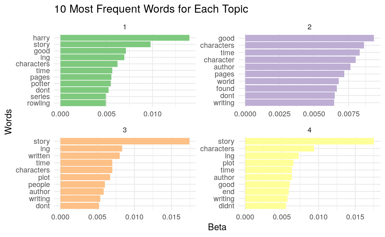
This analysis suggested that all four topics had quite a large number of shared words. Words like “story”, “good”, “writing”, “time”, “plot” and “characters” appeared across most of the topics. Topic 1 appears to uniquely contain a number of words related to the Harry Potter series (“Harry”, “Potter”, “Series”, “Rowling”), while Topics 2, 3 and 4 appeared largely similar.
Show code
# Remove "story," "character", "characters", "didnt", "dont", "page","pages" from the reviews data
filter_words <- review_topics %>%
  filter(!grepl("story|character|characters|didnt|dont|page|pages", term))

# Recreate the graphs of the top terms
new_top_terms <- filter_words %>%
  group_by(topic) %>%
  slice_max(beta, n = 10) %>%
  ungroup() %>%
  arrange(topic, -beta)

new_top_terms %>%
  mutate(term = reorder_within(term, beta, topic)) %>%
  ggplot(aes(beta, term, fill = factor(topic))) +
  geom_col(show.legend = FALSE) +
  facet_wrap(~ topic, scales = "free") +
  scale_fill_brewer(palette = "Accent") +
  labs(title = "10 Most Frequent Words For Each Topic (2.0)",
       x = "Beta",
       y="Words") +
  scale_y_reordered() +
  theme_minimal()
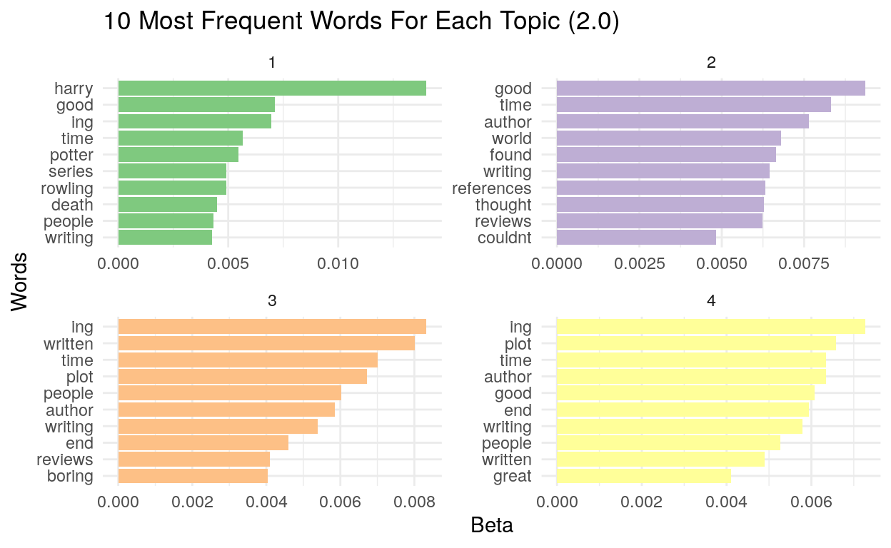
We further removed “writing,” “written,” “author” and “couldn’t.”
Show code
filter_words <- filter_words %>%
  filter(!grepl("writing|written|author|couldnt", term))

# Recreate the graphs of the top terms
new_top_terms <- filter_words %>%
  group_by(topic) %>%
  slice_max(beta, n = 10) %>%
  ungroup() %>%
  arrange(topic, -beta)

new_top_terms %>%
  mutate(term = reorder_within(term, beta, topic)) %>%
  ggplot(aes(beta, term, fill = factor(topic))) +
  geom_col(show.legend = FALSE) +
  facet_wrap(~ topic, scales = "free") +
  scale_fill_brewer(palette = "Accent") +
  labs(title = "10 Most Frequent Words for Each Topic (3.0)",
       x = "Beta",
       y="Words") +
  scale_y_reordered() +
  theme_minimal()
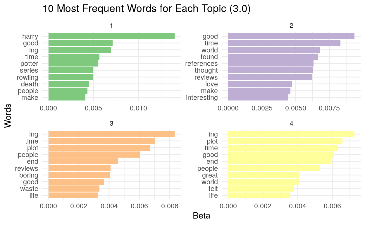
There seemed to be no patterns even after we removed words that were shared with equal frequency across all topics.
Pairwise comparison
To supplement our analysis, we decided to analyze the terms for which the difference between two topics was greatest. Unlike the plots of the top terms for each topic, this analysis allows for the direct comparison of two topics (a pairwise comparison). This would yield terms that are most clearly and uniquely associated with one topic or the other. To automate these pairwise comparisons, we wrote a function that takes in any two topics and produces a plot of the difference in beta values, as represented using the log-ratio function.
The following plots represent the six comparisons made among the four topics.
Show code
# Function to automate pairwise comparisons
pairwise_comparison <- function(topicA, topicB) {
  wide_beta <- review_topics %>%
    mutate(topic = paste0("topic", topic)) %>%
    pivot_wider(names_from = topic, values_from = beta) %>%
    filter(.data[[topicA]] > .001 | .data[[topicB]] > .001) %>%
    mutate(log_ratio = log2(.data[[topicB]] / .data[[topicA]]))

  top_beta_terms <- wide_beta %>%
    slice_max(log_ratio, n = 10)
  bottom_beta_terms <- wide_beta %>%
    slice_min(log_ratio, n = 10)

greatest_diff <- bind_rows(top_beta_terms, bottom_beta_terms)

diff_plot <- greatest_diff %>%
  mutate(term = reorder(term, log_ratio)) %>%
  ggplot(aes(log_ratio, term)) +
  geom_col(show.legend = FALSE, fill = "steelblue3") +
  labs(x = "log-ratio of beta values",
       y = "words") +
  scale_y_reordered()+
  ggtitle(paste0(topicA," (bottom) vs ",topicB," (top)"))+
  theme_ipsum_rc()
diff_plot
}
Show code
pairwise_comparison("topic1", "topic2")
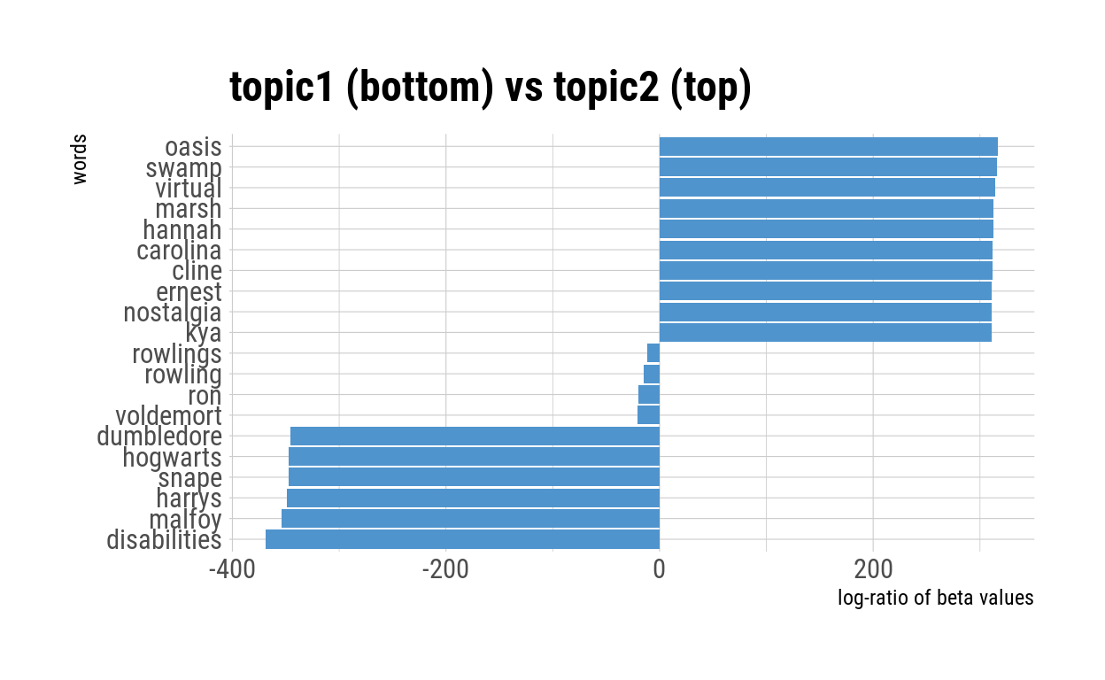
The first comparison of Topic 1 and Topic 2 reveals that many of the unique words from Topic 1 are from the Harry Potter series. Character names, such as Dumbledore, Harry and Snape dominated the comparison, while Topic 2 most uniquely contained the characters and locations of the adult fiction books. Given that the two Harry Potter books contributed less than 10% of the total negative reviews, why did Harry Potter reviews generate a distinct topic? It’s possible that characters were named more in these book reviews than in reviews of other books.
Unlike Topic 1, Topic 2 seemed to capture a range of words. The comparison between Topic 1 and Topic 2 revealed that Topic 2 had some content-related words, such as “oasis”, “swamp”, “hannah” and “carolina”.
Show code
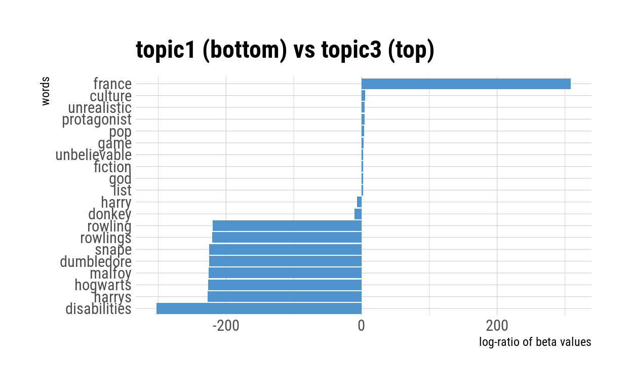
pairwise_comparison("topic1", "topic3")
Show code
pairwise_comparison("topic1", "topic4")
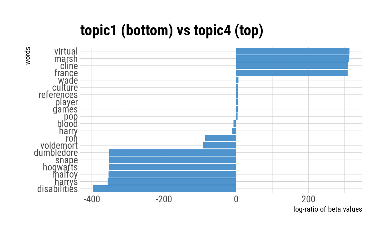
The pairwise comparisons between Topic 1 and 3, and Topic 1 and 4 also reinforce what was found in the comparison between Topic 1 and 2. Interestingly, the latter two comparisons (1 vs. 3 and 1 vs. 4) suggested that the log-ratio of the gamma values were small for most of their top ten words—and that a number of these words appeared to be criticisms of the book’s story structure (“unbelievable”, “protagonist”, “fiction”) or the book’s pop cultural references (“pop”, “culture”, “references”, “game”, “games”).
Show code
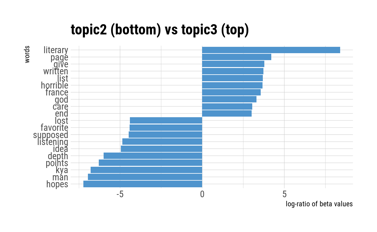
pairwise_comparison("topic2", "topic3")
Show code
pairwise_comparison("topic2", "topic4")
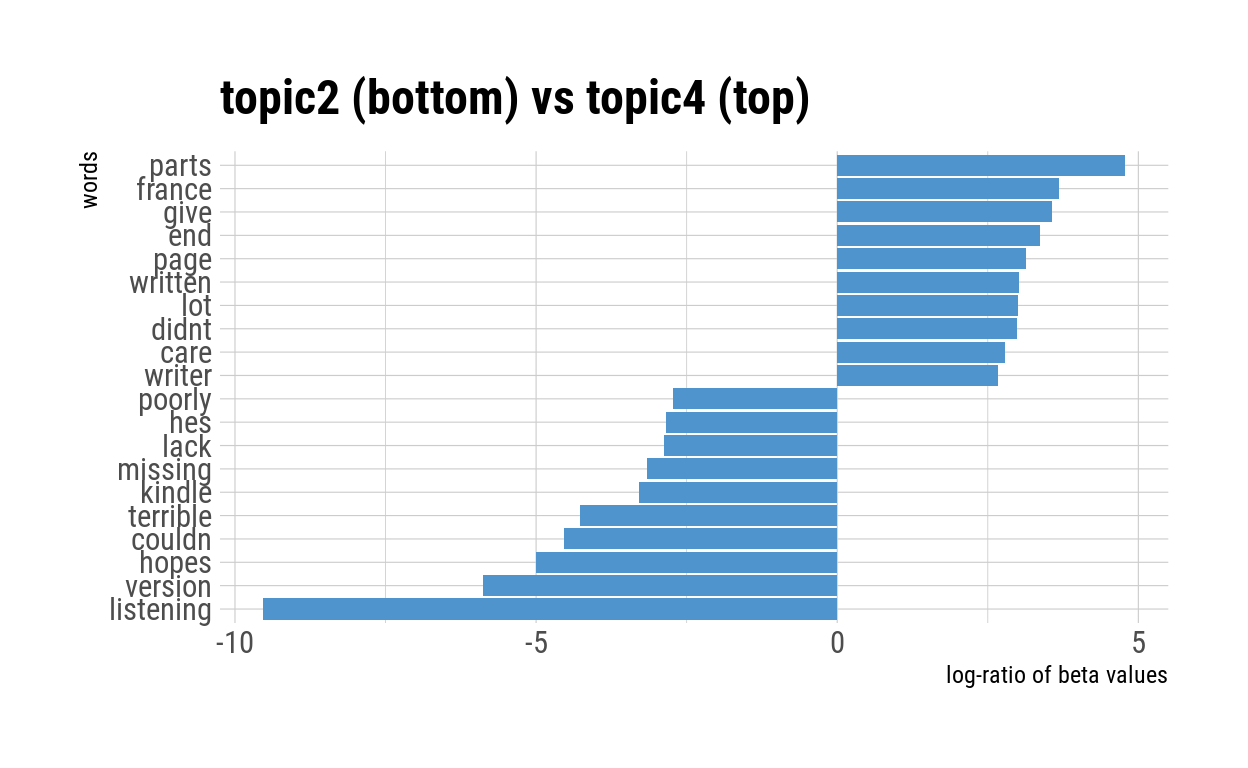
The pairwise comparison between Topic 2 and Topic 3 & 4 did not yield meaningful results.
Show code
pairwise_comparison("topic3", "topic4")
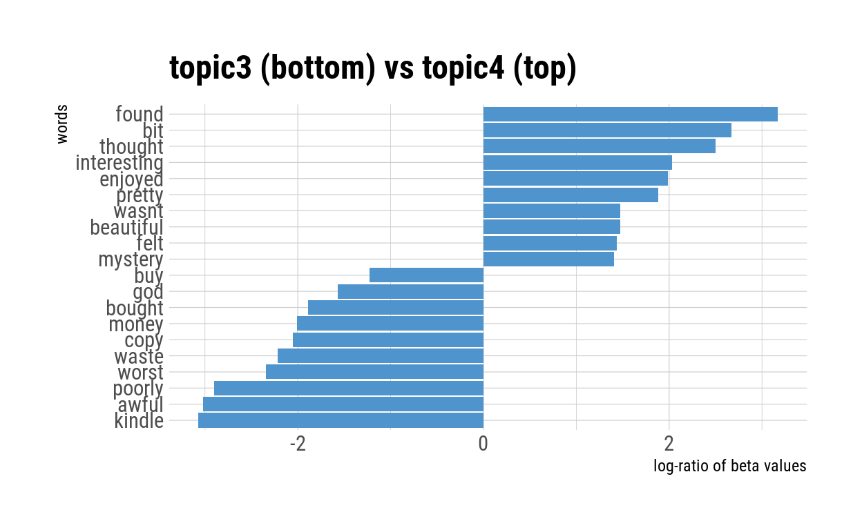
When we examined the pairwise comparison between Topic 3 and Topic 4, no obvious patterns in the content of those words stood out to us. However, we noted that the words in Topic 3 (“awful”, “poorly”, “worst”, “waste”) appeared to be more negative than the words in Topic 4 (“pretty”, “interesting”, “beautiful”, “enjoyed”). Intuitively, it makes sense that Adult 2-Star reviews contained the words from Topic 4, since 2-star reviews may have acknowledged the strengths of a book more than 1-star reviews would have. To illustrate, one Adult 2-star review read: “Although there are some insightful passages, the story does not flow.”
Notably, the pairwise comparison plots differed widely in scale. While the x-axes for the plots comparing Topic 1 and the other topics have a wide range of values (magnitude of 200 to 400), the x-axes for plots comparing the other topics were generally narrower (magnitude of 2 to 10). This makes sense in the context of the kinds of terms shown in the comparison: terms like “Potter”, “Dumbledore” and “Hogwarts” are specific to child book reviews, and hence have extreme log-ratio values.
Per-Document Classification
Next, we explored the probability that each of the above topics would be generated from each category of review (“gamma), and whether there would be any differences in topic assignment based on each category. A greater gamma value for a particular topic within a document means that a greater percentage of the words in that document are drawn from that topic.
Show code
book_lda_4 <- LDA(dtm.new, k = 4, control = list(seed = 1234))

#Using four topics
book_gamma_4 <- tidy(book_lda_4, matrix = "gamma")

book_gamma_4_titled <- book_gamma_4 %>%
  rename(category = document) %>%
  mutate(category = case_when(category == "doc_1" ~ "Adult 1-Star",
                              category == "doc_2" ~ "Adult 2-Star",
                              category == "doc_3" ~ "Child 1-Star",
                              category == "doc_4" ~ "Child 2-Star",))


book_gamma_4_titled %>%
  ggplot(aes(factor(topic), gamma)) +
  geom_boxplot(color = "white") +
  facet_wrap(~ category) +
  labs(x = "topic", y = expression(gamma),
       title = "For each type of review, what's the probability \nthat a certain topic will be generated?") +
  theme_dark() +
  theme(plot.title = element_text(hjust = 0.5))
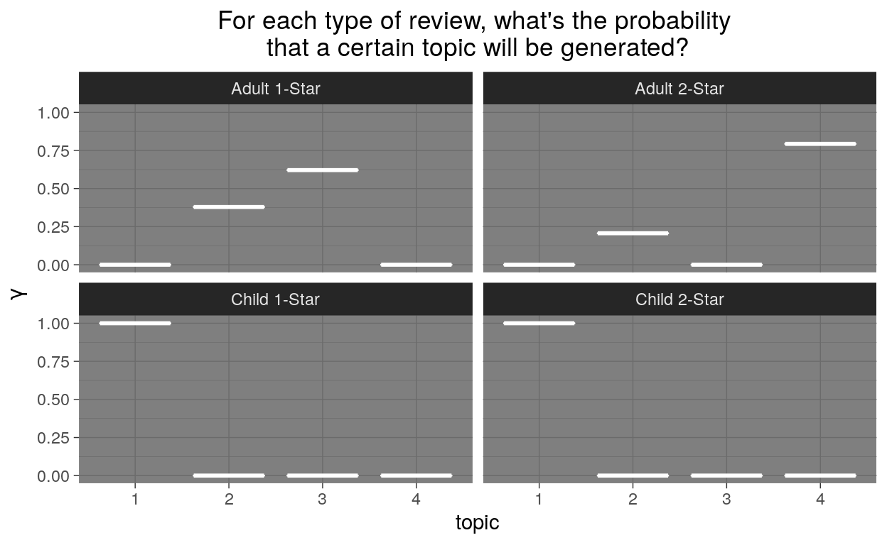
Comparing the findings across categories:
Comparing within 1-star reviews (the left half of the plots), we found that there were no shared topics between the adult book reviews and the child book reviews. The same pattern was found within 2-star reviews.
Comparing within adult fiction reviews (the top plots), we find that Adult 1-Star and 2-Star reviews were split between one shared topic (Topic 2) and one unshared topic (Topic 3 or Topic 4).
Comparing within child book reviews, we find that both contain exactly the same topic.
To identify how words from individual categories were assigned correctly (or otherwise) to the same category, we created a confusion matrix. This shows us the proportion of words correctly assigned to the categories they came from.
Show code
assignments_4 <- augment(book_lda_4, data = dtm.new)

book_classifications <- book_gamma_4_titled %>%
  group_by(category) %>%
  slice_max(gamma) %>%
  ungroup()

book_topics <- book_classifications %>%
  count(category, topic) %>%
  group_by(category) %>%
  slice_max(n, n = 1) %>%
  ungroup() %>%
  transmute(consensus = category, topic)

assignments_4 <- assignments_4 %>%
  inner_join(book_topics, by = c(".topic" = "topic")) %>%
  rename(category_in = document)

assignments_4 %>%
  count(category_in, consensus, wt = count) %>%
  mutate(across(c(category_in, consensus), ~str_wrap(., 20))) %>%
  group_by(category_in) %>%
  mutate(percent = n / sum(n)) %>%
  ggplot(aes(consensus, category_in, fill = percent)) +
  geom_tile() +
  scale_fill_gradient2(high = "darkred", label = percent_format()) +
  theme_minimal() +
  theme(axis.text.x = element_text(angle = 90, hjust = 1),
        panel.grid = element_blank()) +
  labs(x = "Reviews words were assigned to",
       y = "Reviews words came from",
       fill = "% of assignments")
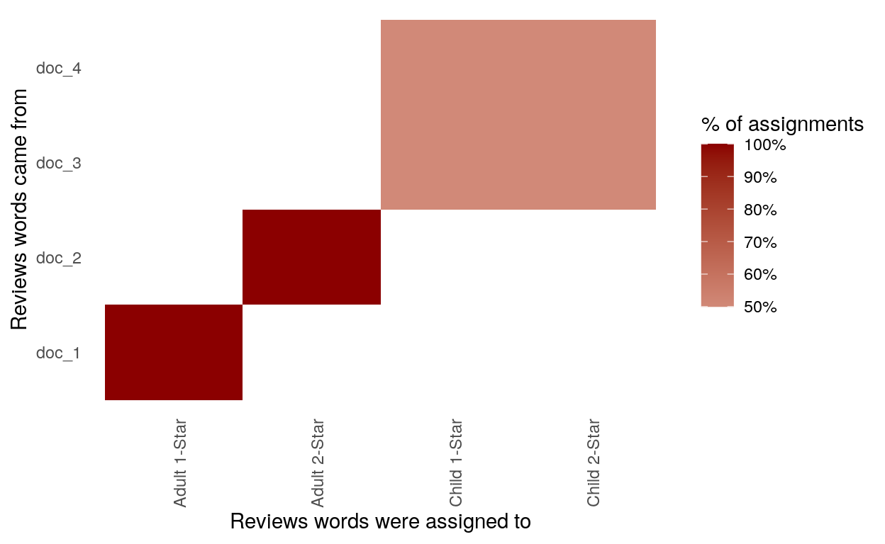
(Note: doc_1 represents Adult 1-Star, doc_2 represents Adult 2-Star, doc_3 represents Child 1-Star and doc_4 represents Child 2-Star)
The confusion matrix reveals that adult fiction review terms were correctly assigned back to their respective categories, but that children’s book reviews were ‘confused’—50% of words from one category were misassigned to the other category, and vice versa! This confirms what we found above, in that Child 1-Star reviews and Child 2-Star reviews have the exact same (single) topic composition.
Conclusions
First, we found that the terms with the greatest beta values within each topic (the words with the greatest probability of being generated from each topic) are largely the same, which suggests that (a) all the reviews in our sample used similar words no matter which category they belonged to and (b) that all the reviews were most likely to have words related to story content (“story”, “good”, “writing”, “time”, “plot” and “characters”). Second, we found that children’s 1-star and 2-star book reviews are far more similar to one another than adult fiction 1-star and 2-star book reviews are. Finally, we found that adult fiction 1-star and adult fiction 2-star book reviews contain a much greater proportion of unshared topics, implying that adult fiction 1-star and adult fiction 2-star book reviews are quite different from one another.
However, there were a few issues with our analysis that raise important considerations for future analyses. First, the presence of two Harry Potter series books may have greatly influenced the topic results found for children’s book reviews. The fact that so many of the Harry Potter characters appeared as important terms may be attributed to the passion of ultra-fans (or ultra-critics!) of the series. (Blog posts showcasing funny negative Harry Potter reviews reaffirm their infamy among Amazon book reviews.) Future work in this area might seek to avoid using books from a series in their sample. Additionally, book review topics are likely to have the book’s particular characters and locations as their most unique terms, which did not help us find differences we were initially interested in (i.e., features of books more broadly).
Despite these limitations, we were still able to identify fairly distinct topics and make connections to our intuitions about various kinds of reviews. Overall, we found LDA topic modeling to be enlightening and engaging. We rate it 5 stars!
Sources
- https://martinctc.github.io/blog/vignette-scraping-amazon-reviews-in-r/
- https://www.tidytextmining.com/topicmodeling.html?q=topic#document-topic-probabilities
- https://sicss.io/2019/materials/day3-text-analysis/topic-modeling/rmarkdown/Topic_Modeling.html#structural-topic-modeling
- https://cfss.uchicago.edu/notes/topic-modeling/
- https://eight2late.wordpress.com/2015/05/27/a-gentle-introduction-to-text-mining-using-r/
- https://eight2late.wordpress.com/2015/09/29/a-gentle-introduction-to-topic-modeling-using-r/