What is art? In the broadest sense art is really just finding an emotional way to tell a complex story. To us, and probably many other data scientists out there, data innately carries with it this artistic quality. While a .csv full of numbers and variables might not have the same accessible and aesthetic qualities we are used to in art, there is nonetheless beauty to be found. With this project we wanted to go beyond our usual representations of data –normal plots and regressions– and present a more artistic way with which to view it.
We chose sentiment analysis data from various books in the Gutenberg Library to serve as the basis of our art (example code for this can be found below). We did this primarily because the sentiment of a book is difficult to plot on a graph or sum nicely into a statistic. It’s not impossible, of course, because we can tell you, for example, that the overall sentiment of The War of the Worlds is -0.393 and the most impactful word is “like.” But we don’t feel like you get the full picture of the book’s sentiments from such statistics. Below, our various attempts at art below will hopefully help bridge that gap between data and understanding. Or, at the very least, we hope to give you a glimpse into the world of data art and the capabilities of R.
library(tidyverse)
library(gutenbergr)

text <- gutenberg_download(36) %>%
  mutate(text = str_to_lower(text, locale = "en"))

afinn <- get_sentiments("afinn")

text_afinn <- text %>%
  unnest_tokens(output = word, input = text, token = "words") %>%
  count(word, sort = TRUE) %>%
  inner_join(afinn, by = "word") %>%
  mutate(prob = n/sum(n),
         impact = abs(n * value)) %>%
  arrange(desc(impact))

sentiment <- sum(text_afinn[["n"]]*text_afinn[["value"]])/sum(text_afinn[["n"]])

sentiment
Before we can make any art, we need to first collect our relevant data. As we mentioned, we are using texts from the Gutenberg Library with the ‘gutenbergr’ package. For these first two pieces, we’re using the book “Stories for Ninon” by Émile Zola. We download our selected text using the ‘gutenberg_download’ function. Once the book is downloaded we “tokenize” it by breaking it into individual words. From this we obtain the affinity score for each word. An affinity score is a -5 to 5 ranking given to each word based on how negative or positive its sentiment is. For example, “breathtaking” gets a rating of 5, while a word like “catastrophic” gets a -4 (We would give an example of a word with a -5 rating, but they are all just a tad too profane for this blog).
Show code
library(tidyverse)
library(gutenbergr)
library(tidytext)

text_num <- 7462

text <- gutenberg_download(text_num) %>%
  mutate(text = str_to_lower(text, locale = "en"))

afinn <- get_sentiments("afinn")

text_afinn <- text %>%
  unnest_tokens(output = word, input = text, token = "words") %>%
  count(word, sort = TRUE) %>%
  inner_join(afinn, by = "word") %>%
  mutate(prob = n/sum(n)) %>%
  arrange(desc(n))

text_neg <- text_afinn %>%
  filter(value < 0) %>%
  arrange(desc(n))

text_pos <- text_afinn %>%
  filter(value > 0) %>%
  arrange(desc(n))
After we calculate individual words’ sentiments, we sum negative, positive, and all values divided by the number of words counted to obtain three different sentiment scores which will be applicable later. These three scores tell us three things: the degree of negative sentiments (how negative the negative elements of the text are), the degree of positive sentiments (how positive the positive elements of the text are), and how positive or negative the text is overall. The last step here multiplies the sentiment score by 10000, rounds it to the nearest whole number, and takes the absolute value as to only output positive values. This may seem odd, but this value will be used to set the “seed” for plots where we use randomization. This makes our art reproducible, because R only uses seeds between 1 and 10000.
The last step before attempting to create art is to build a way to include colors in our masterpieces. We wanted our texts to dictate what colors are used, and since it would be infeasible and impractical to manually sort for colors, we needed to create a way to identify every color within our texts. The process is fairly simple using the ‘stringr’ function ‘str_extract’. All we need to do is provide a list of colors to compare to the text. There are two ways we could do this, the first is to copy and paste a list of common colors. We chose the second option, which is to scrape Wikipedia’s lists of all colors –over 800 total. Next, we go back to our “tokenization” of the text. If we were to only tokenize our text into individual words while looking for color we would miss all of the lovely two and three word color names like ‘international orange’ or ‘deep space sparkle’. Now, we don’t think we will run across many, if any, of these odd colors, but we wanted to be thorough. To ensure we did not lose any colors we “tokenized” the text into n-grams of length 3, (a fancy way of saying three-word chunks). We are, then, left with every three-word combination that appears in the text. This process takes longer and is more computationally demanding than typical one-word tokenizing, but, again, we wanted to be sure to find every possible color. Now, we can compare our Wikipedia list of colors to our text to pull out every matching instance of a color. Corresponding hexadecimal codes are also included from the Wikipedia list in order to account for non-standard colors in R. It is also worth noting here that some of the colors our code pulls out might not be specifically referring to instances of a color being used. The word “bone” for instance might be referring to the color or an actual bone. We intentionally chose to not differentiate the usages of such words. One reason was for practicality, as we have almost no way of systematically identifying how, exactly, words are being used. The second reason is that leaving in these words gives our art pieces more character and variation.
Show code
library(rvest)
library(httr)
library(stringr)

url <- "https://en.wikipedia.org/wiki/List_of_colors:_A%E2%80%93F"
tables <- url %>%
  read_html() %>%
  html_nodes(css = "table")
colors1 <- html_table(tables[[1]], fill = TRUE)

url <- "https://en.wikipedia.org/wiki/List_of_colors:_G%E2%80%93M"
tables <- url %>%
  read_html() %>%
  html_nodes(css = "table")
colors2 <- html_table(tables[[1]], fill = TRUE)

url <- "https://en.wikipedia.org/wiki/List_of_colors:_N%E2%80%93Z"
tables <- url %>%
  read_html() %>%
  html_nodes(css = "table")
colors3 <- html_table(tables[[1]], fill = TRUE)

colors_scrape <- rbind(colors1, colors2, colors3) %>%
  mutate(Name = str_to_lower(Name, locale = "en"),
         Name = str_replace(Name, " \\s*\\([^\\)]+\\)", "")) %>%
  distinct(Name, .keep_all = TRUE)

colors <- colors_scrape %>%
  select(Name)

colors_all <- colors %>%
  summarise(Name = paste0(Name, collapse = "|")) %>%
  as.character(expression())

colors_all <- paste0("\\b(", colors_all, ")\\b")

text_grammed <- text %>%
  unnest_tokens(output = word, input = text,
  token = "ngrams", n = 3)

colors_parsed <- text_grammed %>%
  mutate(Name = str_extract(word, pattern = colors_all)) %>%
  drop_na() %>%
  select(Name)

colors_counted <- colors_parsed %>%
  group_by(Name) %>%
  count() %>%
  ungroup() %>%
  mutate(prob = n/sum(n)) %>%
  arrange(desc(n))

colors_final <- left_join(colors_counted, colors_scrape, by = "Name") %>%
  select(Name, `Hex(RGB)`, n, prob) %>%
  rename(Hex = `Hex(RGB)`)
Randomly GenRating Art
The first art generation tool we created was inspired by the ‘generativeart’ library. This works by using random number generation –based on the sentiment score of the book– and the positive and negative sentiment values calculated previously. So, each artwork produced with this method is unique and dependent on a specific text’s sentiment. This means that texts with more extreme sentiments tend to yield more varied results. If you dig into the formula in the code below, you can see that a sine and cosine function are being multiplied by ‘senti_neg’ and ‘senti_pos’ respectively. So, a larger value for either ‘senti_neg’ or ‘senti_pos’ will make their corresponding function more extreme. We made this graph on desmos as it provides a more intuitive explanation of this interaction. For this piece, we also wanted the colors and titles to be rooted in the text data. The artpiece’s colors are simply the two most common colors to appear in the text. The artpiece’s title is a random sample of three words from the sentiment analysis which are selected based on a word’s proportion of appearance in the text, so words that appear more often are more likely to appear in the title. The lovely generated title for this next piece is “Grand Commit Fan.” For aesthetic reasons we chose to not include the title on our output, though this is toggleable through the function ‘generative_art’ with ‘title = TRUE’. ‘title = TRUE’ will put the generated title in the bottom right corner.
Show code
my_formula <- list(
  x = quote(runif(1, -1, 1) * x_i^2 - senti_neg * sin(y_i^2)),
  y = quote(runif(1, -1, 1) * y_i^2 - senti_pos * cos(x_i^2))
)

color_main <- colors_final %>%
  filter(row_number() == 1) %>%
  select(Hex) %>%
  as.character()

color_background <- colors_final %>%
  filter(row_number() == 2) %>%
  select(Hex) %>%
  as.character()

generative_art <- function(formula = my_formula,
                           polar = TRUE,
                           title = TRUE,
                           main_color = color_main,
                           background_color = color_background) {

  require(tidyverse)
  require(cowplot)

  set.seed(senti)

  df <- seq(from = -pi, to = pi, by = 0.01) %>%
    expand.grid(x_i = ., y_i = .) %>%
    mutate(!!!formula)

    if (polar == TRUE) {
    plot <- df %>%
      ggplot(aes(x = x, y = y)) +
      geom_point(alpha = 0.1, size = 0, shape = 20, color = main_color) +
      theme_void() +
      coord_fixed() +
      coord_polar() +
      theme(
        panel.background = element_rect(fill = background_color, color = background_color),
        plot.background = element_rect(fill = background_color, color = background_color)
        )
  } else {
    plot <- df %>%
      ggplot(aes(x = x, y = y)) +
      geom_point(alpha = 0.1, size = 0, shape = 20, color = main_color) +
      theme_void() +
      coord_fixed() +
      theme(
        panel.background = element_rect(fill = background_color, color = background_color),
        plot.background = element_rect(fill = background_color, color = background_color)
        )
  }

  if(title == TRUE) {

    title <- sample_n(text_afinn, 3, replace = TRUE, weight = prob) %>%
      select(word) %>%
      mutate(word = str_to_title(word))

    title <- title %>%
        summarise(word = paste0(word, collapse = " ")) %>%
        as.character(expression())

    p <- ggdraw(plot) +
      draw_label(title, x = 0.65, y = 0.05, hjust = 0, vjust = 0,
                 fontfamily = "Roboto Condensed", fontface = "plain", color = color_main, size = 10)

    ggsave("genart.png", plot = p)

    p

  } else{
    ggsave("genart.png", plot = plot)

    plot
  }

}

generative_art(polar = TRUE, title = FALSE)
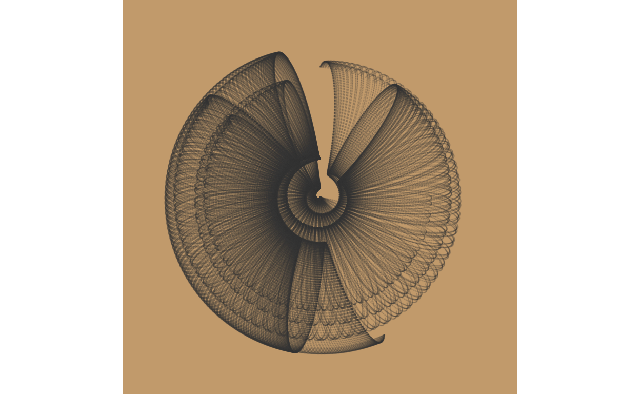
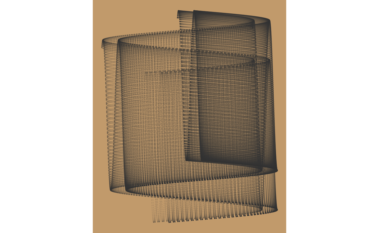
An observant reader might note that the code we used can create art based on polar or cartesian coordinates. The example below uses cartesian coordinates and shows, just like with any form of data visualization, how author inputs can have a massive effect on the final product. All of the code for a non-polar plot is the exact same save for the exclusion of ‘coord_polar()’.
Show code
generative_art(polar = FALSE, title = FALSE)
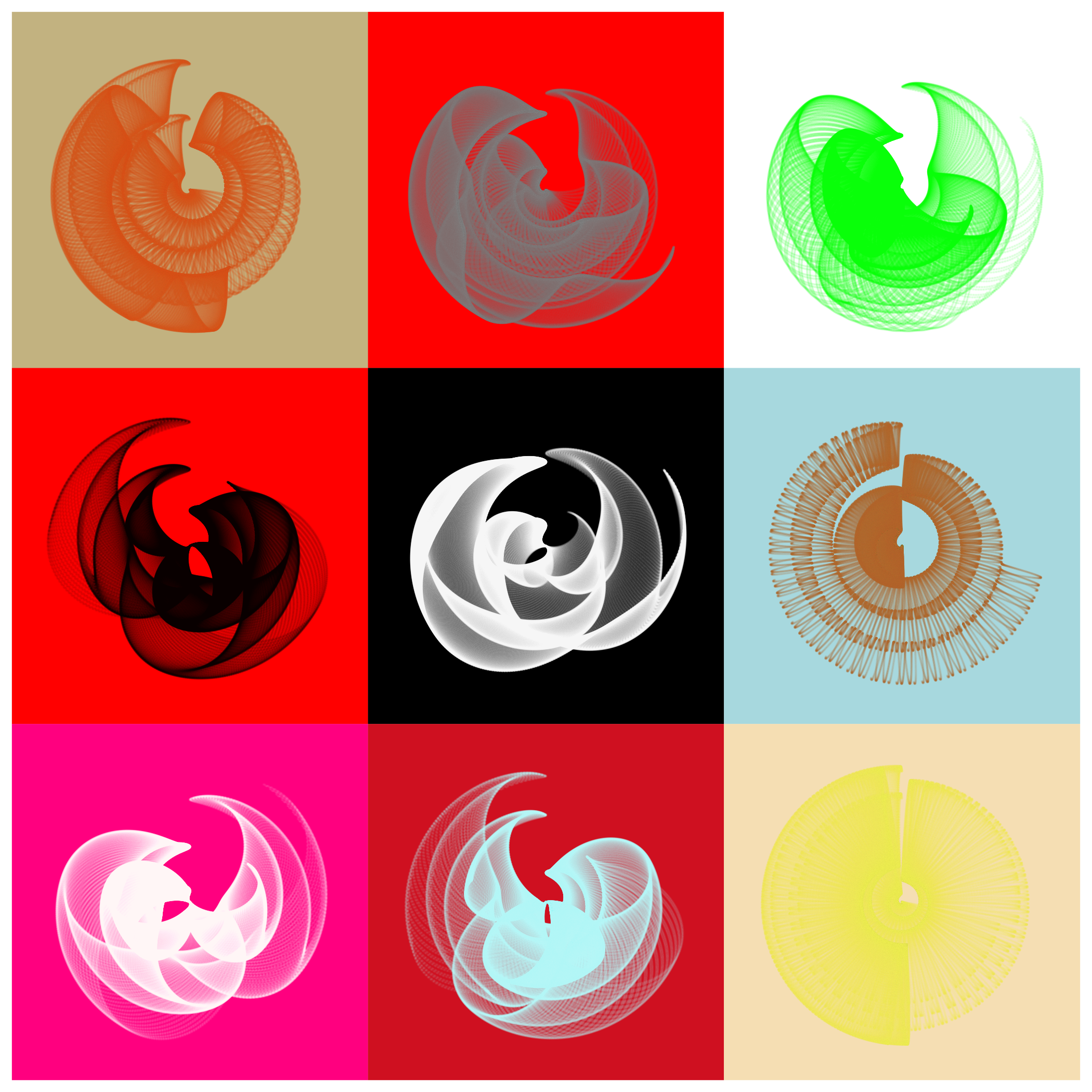
Below are some additional pieces we made with generative art to show you more of a range of potential outputs.

Tunnel aRt
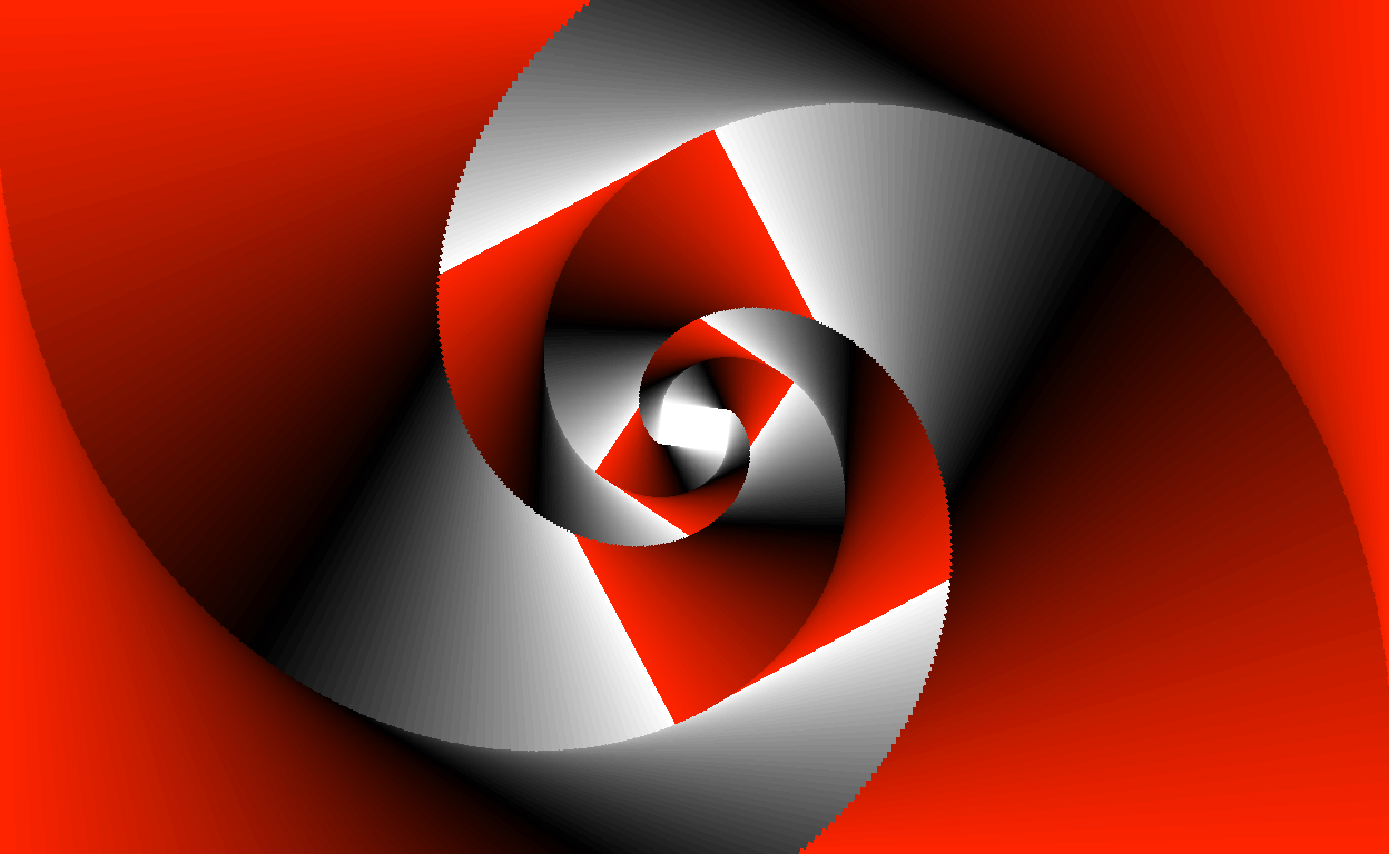
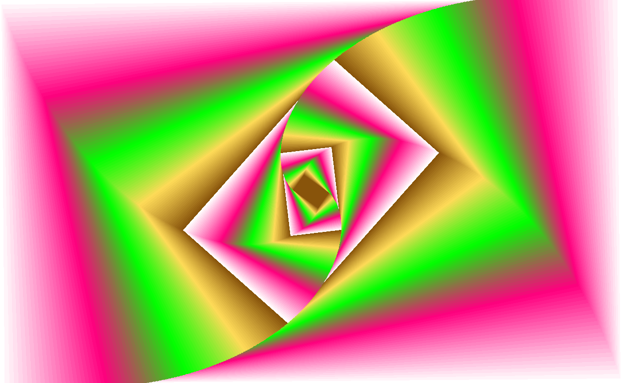
Our next attempt at data art is based off of Jean Fan’s tunnel art. This plot does not use randomization like the ones above. Instead, it takes a series of rectangles which incrementally “push back” and rotate to create a spiral shape. The rotation angle is based upon the raw sentiment score of the text and again, the colors used are pulled from the text. We’re working with a different text than the previous pieces, so we’ll need to re-run most of our previous code. This time we’re working with “The Scarlett Letter” to hopefully get some striking colors. The only difference between these two swirling art pieces is how often the colors repeat. The first has no repetition, while the second has repetition based on the positive sentiment of the piece –the more positive, the more repetition that occurs.
Show code
text_num <- 33

text <- gutenberg_download(text_num) %>%
  mutate(text = str_to_lower(text, locale = "en"))

afinn <- get_sentiments("afinn")

text_afinn <- text %>%
  unnest_tokens(output = word, input = text, token = "words") %>%
  count(word, sort = TRUE) %>%
  inner_join(afinn, by = "word") %>%
  mutate(prob = n/sum(n)) %>%
  arrange(desc(n))

text_neg <- text_afinn %>%
  filter(value < 0) %>%
  arrange(desc(n))

text_pos <- text_afinn %>%
  filter(value > 0) %>%
  arrange(desc(n))

senti_neg <- sum(text_neg[["n"]]*text_neg[["value"]])/sum(text_neg[["n"]])

senti_pos <- sum(text_pos[["n"]]*text_pos[["value"]])/sum(text_pos[["n"]])

senti_raw <- sum(text_afinn[["n"]]*text_afinn[["value"]])/sum(text_afinn[["n"]])

text_grammed <- text %>%
  unnest_tokens(output = word, input = text,
  token = "ngrams", n = 3)

colors_parsed <- text_grammed %>%
  mutate(Name = str_extract(word, pattern = colors_all)) %>%
  drop_na() %>%
  select(Name)

colors_counted <- colors_parsed %>%
  group_by(Name) %>%
  count() %>%
  ungroup() %>%
  mutate(prob = n/sum(n)) %>%
  arrange(desc(n))

colors_final <- left_join(colors_counted, colors_scrape, by = "Name") %>%
  select(Name, `Hex(RGB)`, n, prob) %>%
  rename(Hex = `Hex(RGB)`)
Show code
library(grDevices)
library(grid)

colors_swirl <- colors_final %>%
  slice_head(n = 3)

# Gradient Colors
vp <- viewport(x = 0, y = 0, width = 1, height = 1)
grid.show.viewport(vp)

colors <- colorRampPalette(c(colors_swirl$Hex))(500)

pushViewport(viewport(width = 1, height = 1, angle = 0))

grid.rect(gp = gpar(col = NA, fill = colors[1]))

for(i in 2:500){
  pushViewport(viewport(width = 0.99, height = 0.99, angle = 10*senti_raw))
  grid.rect(gp = gpar(col = NA, fill = colors[i])
  )
}

Show code
vp <- viewport(x = 0, y = 0, width = 1, height = 1)
grid.show.viewport(vp)

colors_swirl <- colors_final %>%
  slice_head(n = 3)

colors <- rep(colorRampPalette(c(colors_swirl$Hex))(100), round(senti_pos) + 1)

pushViewport(viewport(width = 1, height = 1, angle = 0))

grid.rect(gp = gpar(col = NA, fill = colors[1]))

for(i in 2:500){
  pushViewport(viewport(width = 0.99, height = 0.99, angle = 10*senti_raw))
  grid.rect(gp = gpar(col = NA, fill = colors[i])
  )
}
Lastly for the tunnel art, I just could not help myself but to show you the piece made from Alice’s Adventures in Wonderland –the rabbit hole parallels were just too tempting.
Show code
text_num <- 11

text <- gutenberg_download(text_num) %>%
  mutate(text = str_to_lower(text, locale = "en"))

afinn <- get_sentiments("afinn")

text_afinn <- text %>%
  unnest_tokens(output = word, input = text, token = "words") %>%
  count(word, sort = TRUE) %>%
  inner_join(afinn, by = "word") %>%
  mutate(prob = n/sum(n)) %>%
  arrange(desc(n))

text_neg <- text_afinn %>%
  filter(value < 0) %>%
  arrange(desc(n))

text_pos <- text_afinn %>%
  filter(value > 0) %>%
  arrange(desc(n))

senti_neg <- sum(text_neg[["n"]]*text_neg[["value"]])/sum(text_neg[["n"]])

senti_pos <- sum(text_pos[["n"]]*text_pos[["value"]])/sum(text_pos[["n"]])

senti_raw <- sum(text_afinn[["n"]]*text_afinn[["value"]])/sum(text_afinn[["n"]])

text_grammed <- text %>%
  unnest_tokens(output = word, input = text,
  token = "ngrams", n = 3)

colors_parsed <- text_grammed %>%
  mutate(Name = str_extract(word, pattern = colors_all)) %>%
  drop_na() %>%
  select(Name)

colors_counted <- colors_parsed %>%
  group_by(Name) %>%
  count() %>%
  ungroup() %>%
  mutate(prob = n/sum(n)) %>%
  arrange(desc(n))

colors_final <- left_join(colors_counted, colors_scrape, by = "Name") %>%
  select(Name, `Hex(RGB)`, n, prob) %>%
  rename(Hex = `Hex(RGB)`)

vp <- viewport(x = 0, y = 0, width = 1, height = 1)
grid.show.viewport(vp)

colors_swirl <- colors_final %>%
  slice_head(n = 5)

colors <- rep(colorRampPalette(c(colors_swirl$Hex))(100), round(senti_pos) + 1)

pushViewport(viewport(width = 1, height = 1, angle = 0))

grid.rect(gp = gpar(col = NA, fill = colors[1]))

for(i in 2:500){
  pushViewport(viewport(width = 0.99, height = 0.99, angle = 10*senti_raw))
  grid.rect(gp = gpar(col = NA, fill = colors[i])
  )
}
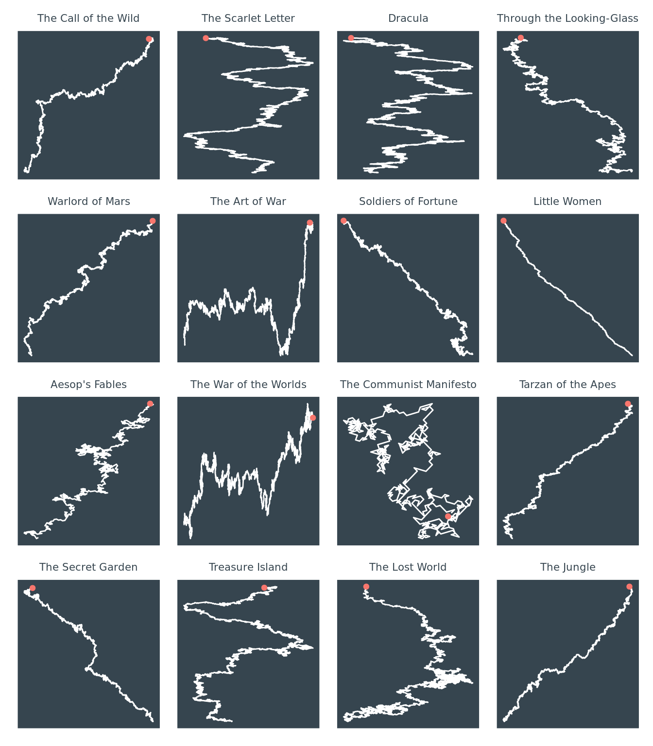
Tracing Sentiment Snakes
Our next attempt at art was a little more straightforward. In the following 16 plots, we plotted every word with a sentiment from the beginning of the text to the end, in order. Starting at the origin (marked with a red dot), a line of length 1 is drawn in the direction corresponding to the sentiment of the word. A line to the left means a negative sentiment. A line to the right means a positive sentiment. The more the line angles down, the stronger the sentiment. For example, a word with the sentiment of +1 would draw a line up and to the right. A word with the sentiment of -5 would draw a line down and to the left. This not only produces visually interesting art, but also helps to convey a story that might otherwise be lost with a typical graph, namely seeing how a text becomes positive or negative over its duration. The general idea for this piece was based on Nadieh Bremer’s visualizations of pi.
Show code
# trying to make something that works vaguely like: https://datatricks.co.uk/the-hidden-art-in-pi

sentiment_snake <- function(text_num){
  text <- gutenberg_download(text_num) %>%
  mutate(text = str_to_lower(text, locale = "en"))

plot_title <- gutenberg_works(gutenberg_id == text_num) %>%
  select(title) %>%
  as.character()

text_afinn_unsort <- text %>%
  unnest_tokens(output = word, input = text, token = "words") %>%
  inner_join(afinn, by = "word")

text_unsort_simp <- text_afinn_unsort %>%
  mutate(value = case_when(value == 1 ~ 1,
                           value == 2 ~ 2,
                           value == -1 ~ -1,
                           value == -2 ~ -2,
                           value %in% 3:5 ~ 3,
                           value %in% -3:-5 ~ -3))

book_coords <- text_unsort_simp %>%
  select(value) %>%
    mutate(sign = sign(value),
         x_coord = cumsum(sign),
         y_coord = cumsum(value))

book_coords_7deg <- text_unsort_simp %>%
  mutate(x_coord = cumsum(case_when(value == 1 ~ .78,
                             value == 2 ~ .97,
                             value == 3 ~ .43,
                             value == -1 ~ -.78,
                             value == -2 ~ -.97,
                             value == -3 ~ -.43)),
         y_coord = cumsum(case_when(value == 1 ~ .62,
                             value == 2 ~ -.22,
                             value == 3 ~ -.9,
                             value == -1 ~ .62,
                             value == -2 ~ -.22,
                             value == -3 ~ -.9)))

df <- tibble(x = 0, y = 0)

ggplot(data = book_coords_7deg, mapping = aes(x = x_coord, y = y_coord)) +
  geom_path(color = "white") +
  geom_point(data = df, mapping = aes(x = x, y = y, color = "red")) +
  ggtitle(plot_title) +
  theme(plot.title = element_text(hjust = 0.5,
                                  family = "Minerva Modern",
                                  size = 8,
                                  color = "#36454f"),
        legend.position = "none",
        axis.title.x = element_blank(),
        axis.text.x = element_blank(),
        axis.ticks.x = element_blank(),
        axis.title.y = element_blank(),
        axis.text.y = element_blank(),
        axis.ticks.y = element_blank(),
        panel.grid.major = element_blank(),
        panel.grid.minor = element_blank(),
        panel.background = element_rect(fill = "#36454f",
                                colour = "#36454f",
                                size = 0.5, linetype = "solid"))
}
Show code
library(patchwork)

sentiment_snake(215) +
  sentiment_snake(33) +
  sentiment_snake(345) +
  sentiment_snake(12) +
  sentiment_snake(68) +
  sentiment_snake(132) +
  sentiment_snake(403) +
  sentiment_snake(514) +
  sentiment_snake(28) +
  sentiment_snake(36) +
  sentiment_snake(61) +
  sentiment_snake(78) +
  sentiment_snake(113) +
  sentiment_snake(120) +
  sentiment_snake(139) +
  sentiment_snake(140) +
  plot_layout(ncol = 4)
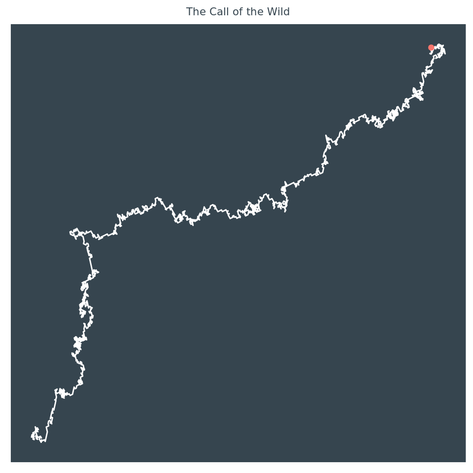
Let’s look at just one example in closer detail so you can better see exactly what is happening. This plot is produced by the text Call of the Wild by Jack London.
Show code
sentiment_snake(215)
If you’re interested seeing what your favorite text looks as one of these plots we made a handy ‘shinyApp’, just type in a title or use the drop-down menu. There is a chance that some plots might not work or that you may experience one or two bugs, but this app is most for fun, so we did not test it extensively.
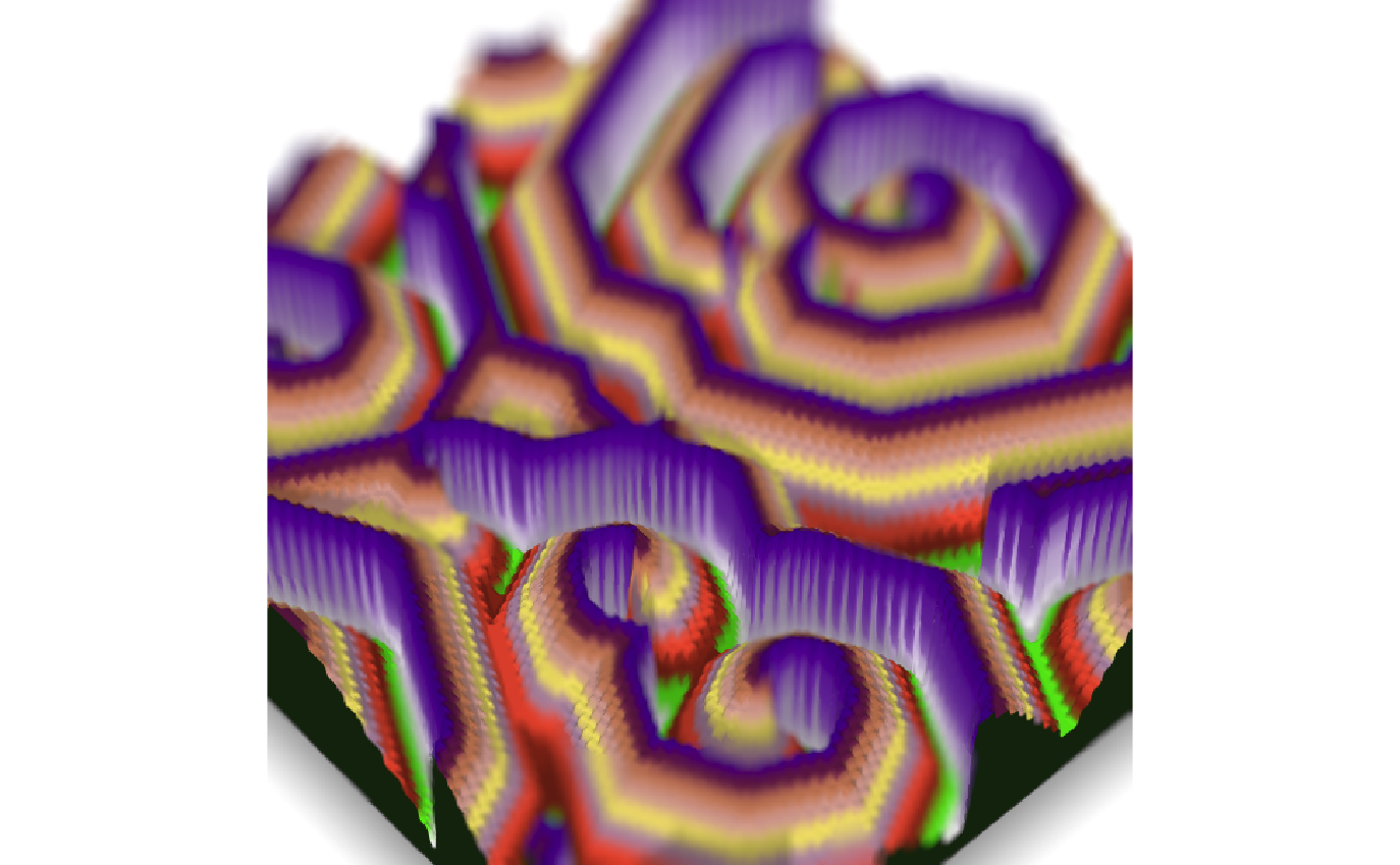
3D Art with rayshader
Our last art generation takes our data art to the next level. The rayshader package contains a save_3Dprint function that can turn 3D models into printable files. This function gives us the potential to turn our data art into a physical object. We generate art for the rayshader models using cellular automata. Cellular automata are a complex mathematical concept that even we cannot fully explain despite having worked with cellular automata to generate this art. Wikipedia defines a cellular automaton as “a discrete model of computation.” Probably a more helpful explanation can be found in youtube videos and tutorials. From our own research we’ve come to understand a cellular automaton as a collection of cells in a grid. The simplest version of a cellular automaton has 2 states, on and off which are indicated by black and white, respectively. A cell that is turned on has the power to decide the state of surrounding cells depending on a neighborhood which is specified in the creation of the automaton. When talking about cellular automata, neighborhoods are certain patterns of cells that are created by mathematical functions. Different neighborhoods give an automaton different visual behaviors. A blog post by Antonio Sánchez Chinchón lists all of the parameters required to produce a cellular automaton in R and also, provides the code that helped us create our art.
Show code
library(rayshader)
library(here)
library(magrittr)
library(raster)
library(sf)
library(dplyr)
library(ggplot2)
library(ambient)
library(rgl)
library("plot3Drgl")
library(rayrender)
library(devtools)
library(textdata)
library(distill)
library(RcppArmadillo)
library(magick)

#cellular automata
library(Rcpp)
library(colourlovers)
library(reshape2)
We start with the same first steps at the previous art generation experiments. After loading all of the necessary libraries, we perform sentiment analysis to help decide our automaton parameters. In this case, we used the nrc lexicon in the get_sentiments function instead of the afinn lexicon. While the afinn lexicon performs a numerical sentiment analysis, the nrc lexicon performs analysis by categorizing words into one of 8 sentiments. We can later use the top sentiment of a text to decide the neighborhood of our automaton. The strongest sentiment, in this case, is anticipation.
Show code
#loading and analyzing text sentiments
text_num_cellauto <- 11 #alice's adventure in wonderland

text_cellauto <- gutenberg_download(text_num_cellauto) %>%
  mutate(text = str_to_lower(text, locale = "en"))

nrc <- get_sentiments("nrc")
data("stop_words")

text_stopped <- text_cellauto %>%
  unnest_tokens(output = word, input = text, token = "words") %>%
  count(word, sort = TRUE) %>%
  anti_join(stop_words, by = "word")

text_nrc <- text_stopped %>%
  inner_join(nrc, by = "word") %>%
  mutate(prop = n/sum(n)) %>%
  arrange(desc(n))

nrc_count <- text_stopped %>%
  inner_join(nrc, by = "word") %>%
  group_by(sentiment) %>%
  mutate(n = sum(n)) %>%
  dplyr::select(!word) %>%
  unique() %>%
  filter(sentiment != "positive") %>%
  filter(sentiment != "negative")

library(gt)

nrc_count %>%
  arrange(desc(n)) %>%
  rename(Count = n, Sentiment = sentiment) %>%
  pivot_wider(values_from = Count, names_from = Sentiment) %>%
  gt()
| anticipation | trust | fear | joy | sadness | anger | surprise | disgust |
|---|---|---|---|---|---|---|---|
| 444 | 422 | 364 | 339 | 327 | 316 | 221 | 191 |
In the next steps we join the Wikipedia color table with the ngram data frame of the selected text. In this example, we look at Alice’s Adventure in Wonderland.
Show code
text_grammed_cellauto <- text_cellauto %>%
  unnest_tokens(output = word, input = text,
  token = "ngrams", n = 3)

colors_parsed_cellauto <- text_grammed_cellauto %>%
  mutate(Name = str_extract(word, pattern = colors_all)) %>%
  drop_na() %>%
  dplyr::select(Name)

colors_counted_cellauto <- colors_parsed_cellauto %>%
  group_by(Name) %>%
  count() %>%
  ungroup() %>%
  mutate(prop = n/sum(n)) %>%
  arrange(desc(n))

colors_final_cellauto <- left_join(colors_counted_cellauto, colors_scrape, by = "Name") %>%
  dplyr::select(Name, `Hex(RGB)`, n, prop) %>%
  rename(Hex = `Hex(RGB)`)
We finally start building our cellular automaton. We pull Antonio Chinchón’s C++ functions from his github to get started. Feeding this code into R is easy. Simply create a new C++ file in R and paste the code from github. Save the C++ file and return to your R project file. Use the sourceCpp() function to feed the C++ code into your R code. Voila! These functions are performing mathematical tasks to ensure the proper operation of our cellular automaton. Honestly, as R coders, the details of these functions purposes are a mystery to us. We only know as much as the code comments tell us. Moving on…
#C++ fxns from aschinchon github

sourceCpp("data/aschinchon_cellularautomata.cpp")
Next, we pull code for two more functions from Antonio Chinchón’s github. The initial_grid function does exactly what the name suggests: create the initial grid for the automaton. Not much creativity is involved in the grid creation, so we leave this code as is from the github. The convolution_indexes function creates neighborhoods to give our automatons. While this code requires creativity, it also requires an understanding of complex mathematical concepts. After extensive research of cellular automata neighborhoods, we chose 8 neighborhood formulas from the original github function based on how well we thought the patterns represented each nrc sentiment (a very scientific and objective process). Now, we have written all of the necessary functions to create our own cellular automata.
#cyclic cellular automata fxns from aschinchon

initial_grid <- function(s, w, h){
  matrix(sample(x = seq_len(s)-1,
               size = w *h,
               replace = TRUE),
         nrow = h,
         ncol = w)}

convolution_indexes <- function(r, n){
  crossing(x = -r:r, y = -r:r) %>%
    mutate(M = ((x != 0) | (y != 0)) * 1,  #Surprise
           N = (abs(x) + abs(y) <= r) * M, #Anticipation
           Cr = ((x == 0) | (y == 0)) * M, #Anger
           S1 = (((x > 0) & (y > 0))|((x < 0) & (y < 0))) * 1, #Fear
           Bl = (abs(x) == abs(y)) * M, #Joy
           D1 = (abs(x) > abs(y)) * M, #Sadness
           Z = ((abs(y) == r) | (x == y)) * M, #Disgust
           TM = ((abs(x) == abs(y)) | abs(x) == r | abs(y) == r) * M) %>% #Trust
    dplyr::select(x, y, matches(n)) %>%
    filter_at(3, all_vars(. > 0)) %>%
    dplyr::select(x,y)
}
We have to create a data frame before we can plot our cellular automaton. We provide the automaton with all of the parameters that Antonio Chinchón’s blog post specifies. To more thoroughly explain each parameter:
range tells the automaton how far each neighborhood extends from a cell. threshold tells the automaton how many different states a cell can reach before the automaton moves on to another cell. states tells the automaton how many different varieties of cells or how many different colors can exist in the plot. We have already discussed the role of the neighborhood in creating the automaton. iter, and abbreviation of iteration, tell the automaton how many times the it should run through the model. Finally, the width and height decide the dimensions of your final plot.
These parameters cannot be given a random set of numbers and be expected to generate an interesting visual pattern. Most number combinations produce what can only be described as color static. Jason of softologyblog provides some number combinations to begin with when trying to produce interesting visuals with cellular automata. We started with combinations that allowed a large number of cell states, because we wanted to include at least the top ten colors mentioned in a text. Plus, more color makes our art pieces more interesting.
Object X creates the automaton’s grid. Object L runs the automaton using a for loop. The larger the specified width and height of your plot, the longer the for loop will take to run. Antonio Chinchón’s github example of an automaton had a width and height of 1500 and took upwards of five minutes to run the for loop. For the sake of experimentation, we kept our dimensions relatively small. Larger dimensions would create higher quality, less pixelated automaton images by including more cells and much smaller cells.
The melt function turns the output of the for loop into a tidy data frame with every row as an observation.
Show code
#create dataframe

range <- 3 #depth of the neighborhood
threshold <- 3 #cell limit
states <- 10 #maximum number of states allowed (algorithm M)
neighborhood <- "N" #pattern of neighboring cells
iter <- 171 #number of iterations

width  <- 150
height <- 150

X <- initial_grid(s = states,
                  w = width,
                  h = height)

L <- convolution_indexes(r = range, n = neighborhood)

for (i in 1:iter){
    X <- iterate_cyclic(X, L, states, threshold)
}

df <- melt(X)
colnames(df) <- c("x","y","v") # to name columns
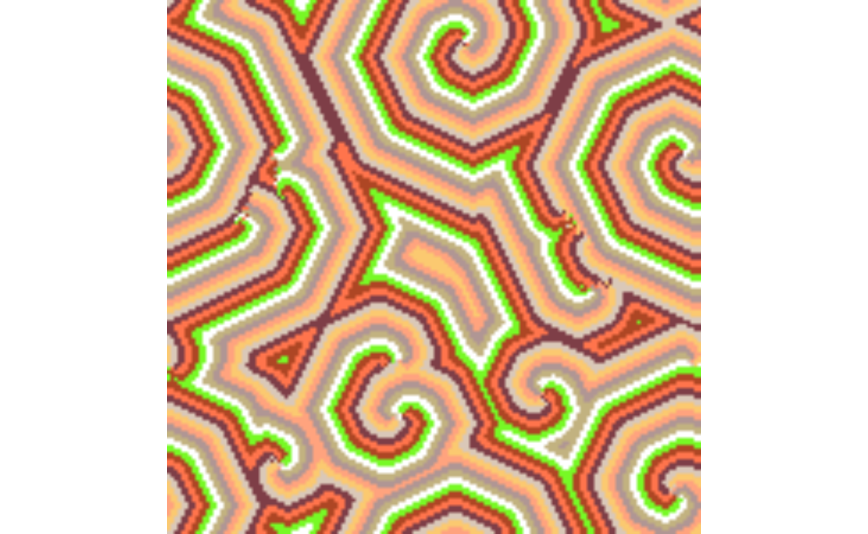
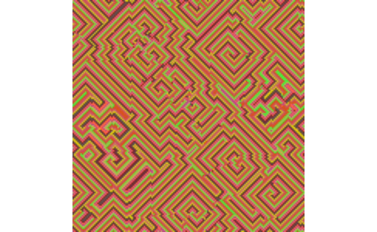
Use the data frame to plot the automaton with the geom_raster function. Within the geom_raster function, interpolate = TRUE smoothens out the plot image, and the theme_nothing function creates an output with the appearance of an image instead of a graph. Once we produced an output that we were happy with, we turned the plot into a ggobject. This object gets put into the rayshader plot_gg function.
Show code
#plot cells

colors <- colors_final_cellauto$Hex

ggobj = ggplot(data = df, aes(x = x, y = y, fill = v)) +
  geom_raster(interpolate = TRUE) +
  coord_equal() +
  scale_fill_gradientn(colours = colors) +
  scale_y_continuous(expand = c(0,0)) +
  scale_x_continuous(expand = c(0,0)) +
  theme_nothing()
ggobj
The rayshader models can only be viewed on a local installation of R. An R studio server will not be able to produce the rgl device window which is necessary to view 3D models. If using a Mac, make sure to download and open XQuartz before running the rayshader code. Macs will not be able to open an rgl device window without XQuartz. Once you have adjusted the rayshader code to produce a model of your liking, use the save_3Dprint function to produce a file that you can take to your local 3D printer, wherever that may be.
Show code
#rayshader

filename_map = tempfile()

plot_gg(ggobj, solid = TRUE, multicore = TRUE,
        fov = 30, zoom = 0.5, theta = 228, phi = 50)
render_depth(focus = 0.50, focallength = 200)
Show code
knitr::include_graphics("images/000067.png")
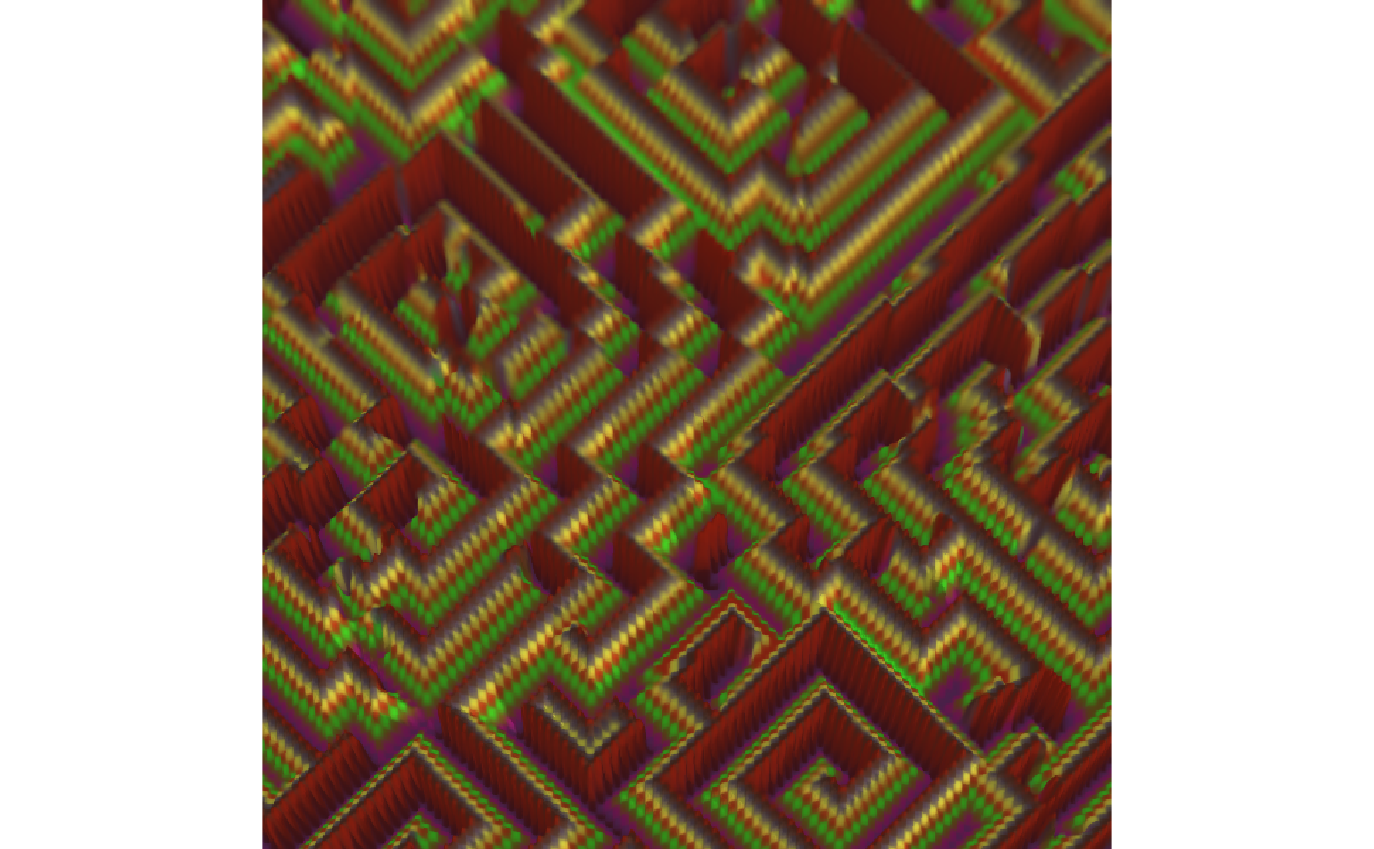
Here’s one more example with The Strange Case of Dr. Jekyll and Mr. Hyde! The strongest sentiment here is anger.
Show code
#loading and analyzing text sentiments
text_num_cellauto2 <- 42 #The Strange Case of Dr. Jekyll and Mr. Hyde

text_cellauto2 <- gutenberg_download(text_num_cellauto2) %>%
  mutate(text = str_to_lower(text, locale = "en"))

nrc2 <- get_sentiments("nrc")
data("stop_words")

text_stopped2 <- text_cellauto2 %>%
  unnest_tokens(output = word, input = text, token = "words") %>%
  count(word, sort = TRUE) %>%
  anti_join(stop_words, by = "word")

text_nrc2 <- text_stopped2 %>%
  inner_join(nrc, by = "word") %>%
  mutate(prop = n/sum(n)) %>%
  arrange(desc(n))

nrc_count2 <- text_stopped2 %>%
  inner_join(nrc, by = "word") %>%
  group_by(sentiment) %>%
  mutate(n = sum(n)) %>%
  dplyr::select(!word) %>%
  unique() %>%
  filter(sentiment != "positive") %>%
  filter(sentiment != "negative")


#creating color correspondence
text_grammed_cellauto2 <- text_cellauto2 %>%
  unnest_tokens(output = word, input = text,
  token = "ngrams", n = 3)

colors_parsed_cellauto2 <- text_grammed_cellauto2 %>%
  mutate(Name = str_extract(word, pattern = colors_all)) %>%
  drop_na() %>%
  dplyr::select(Name)

colors_counted_cellauto2 <- colors_parsed_cellauto2 %>%
  group_by(Name) %>%
  count() %>%
  ungroup() %>%
  mutate(prop = n/sum(n)) %>%
  arrange(desc(n))

colors_final_cellauto2 <- left_join(colors_counted_cellauto2, colors_scrape, by = "Name") %>%
  dplyr::select(Name, `Hex(RGB)`, n, prop) %>%
  rename(Hex = `Hex(RGB)`)

range <- 1 #depth of the neighborhood
threshold <- 1 #cell limit
states <- 10 #maximum number of states allowed (algorithm M)
neighborhood <- "Cr" #pattern of neighboring cells
iter <- 171 #number of iterations

width  <- 150
height <- 150

X_ <- initial_grid(s = states,
                  w = width,
                  h = height)

L_ <- convolution_indexes(r = range, n = neighborhood)

for (i in 1:iter){
  sourceCpp(here("./_posts/2021-03-07-mini-project-2-instructions/data/aschinchon_cellularautomata.cpp"))
    X_ <- iterate_cyclic(X_, L_, states, threshold)
}

df2 <- melt(X_)
colnames(df2) <- c("x","y","v") # to name columns

colors2 <- colors_final_cellauto2$Hex

ggobj2 = ggplot(data = df2, aes(x = x, y = y, fill = v)) +
  geom_raster(interpolate = TRUE) +
  coord_equal() +
  scale_fill_gradientn(colours = colors2) +
  scale_y_continuous(expand = c(0,0)) +
  scale_x_continuous(expand = c(0,0)) +
  theme_nothing()
ggobj2
Show code
plot_gg(ggobj2, solid = TRUE, multicore = TRUE,
        fov = 30, zoom = 0.4, theta = 180, phi = 75)
render_depth(focus = 0.55, focallength = 200)
Show code
knitr::include_graphics("images/000017.png")
Time permitting, we would have loved to take this project a step further in terms of reproducibility. We believe that a function that automates the creation of a text data cellular automaton is a time-consuming but worthwhile project for the future. In our vision, the function requires a single input: a gutenbergr text number. The function would perform the same nrc text analysis we already wrote to identify the given text’s strongest sentiment. The function would then choose the neighborhood that we would have liked to match to the identified popular sentiment. Finally, the function would choose the cellular automaton’s 10 colors using the color and text code we’ve already written. There would be two outputs: the data frame and the rayshader plot. In this imagined function, the number of range, states, and threshold would always stay the same. The iterations, width, and height would be optional, adjustable inputs for the function. Ultimately, we would be able to produce unique art pieces with one line of code, and we would be able to make a physical copy with just one more line. All we would need is two lines of code to become an artist! Imagine that…