Political Corruption by Region
Political corruption is an issue that significantly affects the functioning of nations around the world, but it comes in different forms and varies in prevalence. Corruption can often carry many definitions, which can be tricky when analyzing potential factors that cause it. A standard definition of corruption is when a person or people take advantage of public office for personal gain (Jain, 2008). Many researchers have explored how different social norms in different areas influence corruption (Dong et al., 2009; Köbis et al., 2017). To investigate, we decided to use the political corruption data collected by the Varieties of Democracy Institute (V-Dem) to investigate.
V-Dem is one of the largest social science databases. It includes many novel measures, like political corruption, in order to provide a more nuanced picture of democracy. By differentiating between five principles of democracy (electoral, liberal, participatory, deliberative, and egalitarian), V-Dem shows that democracy is about more than just the presence of elections. The specific V-Dem dataset we started out with (v11, from March 2021) has 27192 observations and 4176 variables. Each row in the dataset represents one of 202 countries in a given year, from 1798-2020. Because it is so large, we immediately decided to look at a subset of the data (179 observations/countries and 17 variables) from 2018.
Wanting to isolate the relationship of political corruption to different social norms, we were interested to see how corruption differs by region. Because the vdem dataset coded regions as numbers, this required some renaming, and merging on our end. To see how political corruption is affected by region, we created a plot that highlights the different scores by region as well as the mean and standard deviation of political corruption scores for each region.
Show code
#rename regions
e_regiongeo <- c(1, 2, 3, 4, 5, 6, 7, 8, 9, 10, 11, 12, 13,
                 14, 15, 16, 17, 18, 19)
region <- c("Western Europe", "Northern Europe", "Southern Europe","Eastern Europe",
            "Northern Africa", "Western Africa", "Middle Africa", "Eastern Africa",
            "Southern Africa", "Western Asia", "Central Asia", "Eastern Asia",
            "South-Eastern Asia", "Southern Asia", "Oceania", "North America",
            "Central America", "South America", "Caribbean")
region.recode <- data.frame(e_regiongeo, region)
names(vdem)[names(vdem) == "country_name"] <- "Country"
#merge new region names to dataset
vdem <- vdem %>%
  left_join(region.recode, by = c("e_regiongeo")) %>%
  select(-c(e_regiongeo))
#plot regions
RegionPlot<- ggplot(vdem, aes(x = region, y = v2x_corr)) +
  geom_point() +
  stat_summary(fun.data = mean_sdl, fun.args = list(mult=1),
                 geom="pointrange", color="red", alpha = 0.5) +
  theme_linedraw() +
  labs(x = "Region", y = "Political Corruption Score",
       title = "Political Corruption by Region (2018)",
       subtitle = "Including the mean and standard deviation.")+
  theme(axis.text.x = element_text(angle = -90, hjust = 0, vjust = .7))
RegionPlot
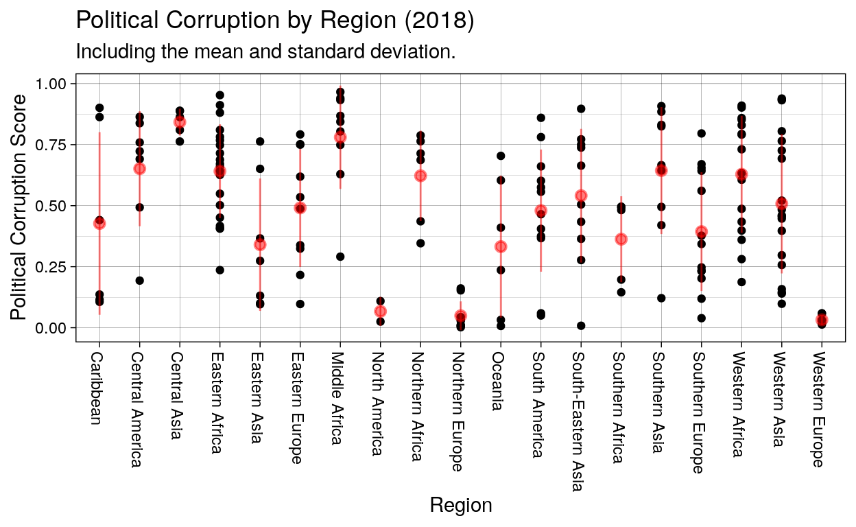
This plot highlights the overall political corruption scores across regions in the war. Looking at the plot, it is clear that region and similar norms and histories do not necessarily result in similar corruption scores as we expected. The red dot and error bars represent the mean and standard deviation of the overall political corruption of each region. Since most of the error bars cover most of the points in each region, it is clear that region does not determine political corruption. Recognizing this, we decided to change course. We decided to choose one region, Latin America, and try to understand what factors contributed to different corruption ratings; Latin America covers countries in South America, Central America, and the Caribbean. It is well acknowledged in political corruption literature that a country or region’s colonial past plays a considerable role as the roots of political corruption in that country or region and is specifically present in Latin America (Angeles and Neanidis 2015; Warf and Stewart 2016; Sokoloff and Engerman 2000; Acemoglu et al. 2001; Bulmer-Thomas 2003; Coatsworth 2008). Noting this, we recognized that there are still diverse histories of colonization and exploitation of each of the nations in Latin America, despite these countries being in the same region. So, to further narrow our focus and control for similar colonial histories, we decided to explore Latin American countries that are (1) former Spanish colonies and (2) gained their independence in the early 1800s.
Show code
#isolate the 16 countries we are interested in
Country <- c("Argentina", "Bolivia", "Chile", "Colombia", "Costa Rica", "Ecuador", "El Salvador",
             "Guatemala", "Haiti", "Hondouras", "Mexico", "Nicaragua", "Panama", "Paraguay", "Peru",
             "Uruguay", "Venezuela")
spain.colonized <- TRUE
colonies <- data.frame(Country, spain.colonized)
vdem <- vdem %>%
  left_join(colonies, by = "Country")%>%
  mutate(spain.colonized = replace_na(spain.colonized, FALSE))

vdem_spanish <- vdem %>%
  filter(spain.colonized == TRUE) %>%
  arrange(desc(v2x_corr))
#plot region plot highlighting the subset of countries we are interested in
RegionPlot2 <- ggplot(vdem, aes(x = region, y = v2x_corr)) +
  geom_point(aes(color = spain.colonized)) +
  theme_linedraw() +
  labs(x = "Region", y = "Political Corruption Score",
       title = "Political Corruption by Region (2018)",
       color='Former Spanish Colony that Gained Independence Early 1800s') +
  theme(axis.text.x = element_text(angle = -90, hjust = 0, vjust = .5),
        legend.position="top") +
  scale_color_manual(values=c('#000000','#00A8FF'))
RegionPlot2
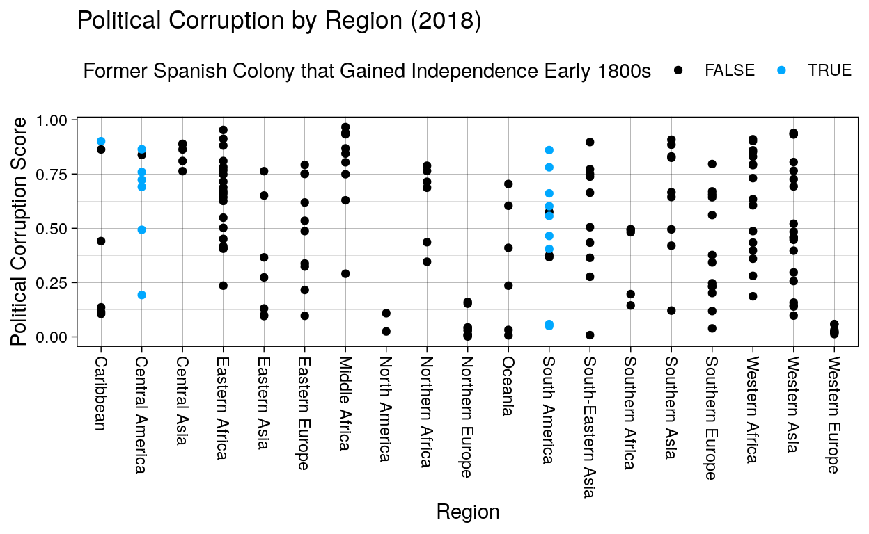
The region plot highlights those specific countries, which clearly still have a variety of corruption ratings but have a very similar past of colonialism that they had to overcome. This brings us to our final and main research question: How do the corruption scores of countries that gained their independence from Spain around the same time period compare, and what variables contribute to or reflect their differences?
How Political Corruption Compares In Former Spanish Colonies
To answer this question, we focused on data from 2018 because it is fairly recent but before the start of the COVID-19 pandemic, which dominated global and domestic politics. V-Dem’s overall political corruption score is a measure of the pervasiveness of overall political corruption in a country, with values ranging from 0 to 1. The higher the political corruption score, the more pervasive political corruption is in a country. To visually compare the political corruption of these countries, we created a plot of not only each country’s overall political corruption score, but of the four components that make that score: executive corruption, public sector corruption, legislative corruption, and judicial corruption. However, to properly compare, we had to re-code the latter two corruption variables since were coded in the dataset as their z-score, and put the data in tidy formatting.
Show code
#create variable that ranks countries from highest corruption score to lowest
vdem_spanish$Rank <- rank(vdem_spanish$v2x_corr)
#revalue the judicial and legislative corruption scores from z-scores to 0-1 range
vdem_spanish$v2jucorrdc <- (1-(pnorm(vdem_spanish$v2jucorrdc, 0, 1)))
vdem_spanish$v2jucorrdc <- round(vdem_spanish$v2jucorrdc, digits = 3)
vdem_spanish$v2lgcrrpt <- (1-(pnorm(vdem_spanish$v2lgcrrpt, 0, 1)))
vdem_spanish$v2lgcrrpt <- round(vdem_spanish$v2lgcrrpt, digits = 3)
#create tidy dataset to plot with
corruption.tidy <- pivot_longer(vdem_spanish, cols = c(v2x_corr, v2x_execorr, v2x_pubcorr, v2lgcrrpt, v2jucorrdc),
                                names_to = "Corruption.Type",
                                values_to = "Corruption.Score") %>%
  select(Country, year, Corruption.Type, Corruption.Score, Rank, e_migdppc, v2x_gender) %>%
  arrange(desc(Rank))
highlight.v2x_corr <- corruption.tidy %>%
  filter(Corruption.Type == "v2x_corr")
#find mean of all overall political corruption scores to add to plot
mean_corr <- mean(vdem_spanish$v2x_corr)
This plot looks at the political corruption prevalence in these countries. The large magenta dots represent the overall political corruption score, and the other dots represent corruption scores for specific types of corruption that make up the overall score.
Show code
CorruptionPlot <- ggplot(corruption.tidy, aes(x = reorder(Country, Rank), y = Corruption.Score)) +
  geom_hline(aes(yintercept = 0.57, linetype = "mean of overall corruption")) +
  geom_point(data = highlight.v2x_corr,
             aes(y = Corruption.Score, color = Corruption.Type),
                 size = 4) +
  geom_point(aes(color = Corruption.Type)) +
  scale_color_manual(name = "Corruption Type",
                     labels = c("judicial",
                                "legislative",
                                "overall",
                                "executive",
                                "public sector"),
                     values=c("#FFD400", "#0571B0", "#AA4371", "#44CF7C", "#E66101")) +
  theme_linedraw() +
  theme(axis.text.x = element_text(angle = -90, hjust = 0, vjust = .5)) +
  labs(x = "Country",
       y = "Political Corruption Score",
       title = "2018 Political Corruption Scores of Former Spanish Colonies",
       subtitle = "Specifically, Spanish colonies that became independent in the early 1800s.") +
  scale_y_continuous(breaks = sort(c(seq(min(0), max(1), length.out=5), 0.57))) +
  scale_linetype_manual(name ="", values = c('dashed'))
CorruptionPlot
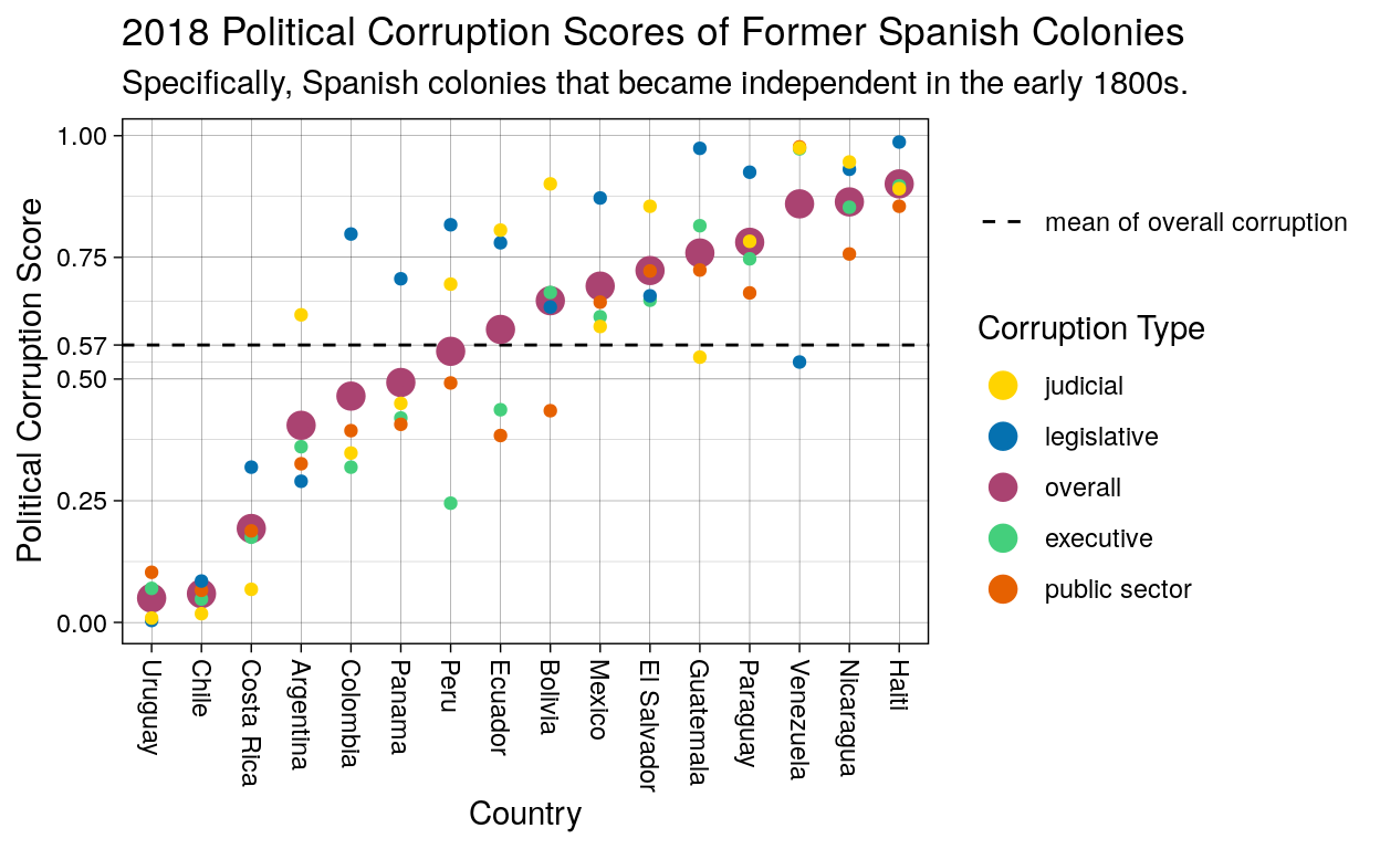
Despite the fact that these 16 countries have similar colonial histories, there is considerable variation in the overall corruption scores across the countries; the overall corruption scores span nearly the whole range of possible V-Dem dataset corruption values. Uruguay has an overall corruption score of 0.050, while Haiti has an overall corruption score of 0.901. At the same time, most of these countries have an overall corruption score above 0.5 (the mean is 0.5665), suggesting that corruption is quite pervasive among countries formerly colonized by Spain, supporting the literature. This plot also illuminates specific types of corruption that are noticeably less/more problematic in certain countries. For instance, Venezuela’s overall corruption score is quite high (0.860), but its legislative corruption score is much lower (0.535). This highlights and supports our assumption that despite these countries having very similarly histories and timelines, there are other components at play.
Wanting to understand the relationship of corruption to other components of the political and economic components/observations of each country, we decided to look at some other V-Dem variables to try and understand these differences. The new variables included GDP per capita, media bias, and political equality for different demographics.
Show code
vdem_spanish %>%
  select(-c(year, region, spain.colonized, Rank)) %>%
  kbl(caption = "2018 Variable Scores of Countries of Former Spanish Colonies",
      col.names = c("Country",
                    "Overall Politcal Corruption Score",
                    "Executive Corruption",
                    "Public Sector Corruption",
                    "Legislative Corruption",
                    "Judicial Corruption",
                    "Government Censorship of Media",
                    "Media Bias",
                    "Educational Equality",
                    "Party Institutionalization",
                    "Power by Socioeconomic Status",
                    "Women Political Empowerment",
                    "Distribution of Resources",
                    "GDP Per Capita"
                    )) %>%
  kable_minimal() %>%
  kable_styling(latex_options = "scale_down") %>%
  scroll_box(width = "1000px", height = "100%") %>%
  footnote(general = "This data was collected from v-dem.net")
| Country | Overall Politcal Corruption Score | Executive Corruption | Public Sector Corruption | Legislative Corruption | Judicial Corruption | Government Censorship of Media | Media Bias | Educational Equality | Party Institutionalization | Power by Socioeconomic Status | Women Political Empowerment | Distribution of Resources | GDP Per Capita |
|---|---|---|---|---|---|---|---|---|---|---|---|---|---|
| Haiti | 0.901 | 0.897 | 0.855 | 0.987 | 0.891 | 0.621 | 1.741 | -1.918 | 0.201 | -0.854 | 0.468 | 0.089 | 1729.04 |
| Nicaragua | 0.864 | 0.853 | 0.757 | 0.931 | 0.946 | -1.565 | 0.034 | -0.687 | 0.581 | -0.462 | 0.714 | 0.381 | 4952.48 |
| Venezuela | 0.860 | 0.973 | 0.977 | 0.535 | 0.975 | -2.493 | -0.145 | -1.350 | 0.496 | 1.116 | 0.761 | 0.083 | 10709.95 |
| Paraguay | 0.781 | 0.747 | 0.677 | 0.925 | 0.783 | 1.575 | 1.145 | -1.694 | 0.539 | -0.160 | 0.718 | 0.148 | 9338.95 |
| Guatemala | 0.759 | 0.815 | 0.724 | 0.974 | 0.545 | 0.666 | 0.937 | -1.013 | 0.348 | 0.087 | 0.728 | 0.228 | 7402.11 |
| El Salvador | 0.723 | 0.662 | 0.722 | 0.671 | 0.855 | 1.160 | 1.197 | -1.383 | 0.897 | -0.524 | 0.750 | 0.272 | 8598.20 |
| Mexico | 0.691 | 0.628 | 0.658 | 0.872 | 0.608 | 1.083 | 1.621 | -0.660 | 0.861 | 0.520 | 0.832 | 0.358 | 16494.08 |
| Bolivia | 0.661 | 0.678 | 0.435 | 0.648 | 0.901 | 0.206 | 1.097 | -0.982 | 0.700 | 1.710 | 0.805 | 0.356 | 6695.77 |
| Ecuador | 0.602 | 0.437 | 0.384 | 0.780 | 0.806 | 2.055 | 0.856 | 0.767 | 0.378 | 1.018 | 0.866 | 0.645 | 10638.83 |
| Peru | 0.557 | 0.245 | 0.492 | 0.817 | 0.695 | 2.199 | 1.524 | -0.582 | 0.412 | 0.970 | 0.852 | 0.397 | 12310.08 |
| Panama | 0.493 | 0.420 | 0.407 | 0.706 | 0.450 | 1.003 | 1.129 | 0.510 | 0.671 | 0.033 | 0.821 | 0.693 | 22637.15 |
| Colombia | 0.465 | 0.319 | 0.394 | 0.798 | 0.348 | 1.364 | 1.139 | -0.446 | 0.537 | 0.024 | 0.758 | 0.364 | 13545.05 |
| Argentina | 0.405 | 0.361 | 0.326 | 0.290 | 0.632 | 1.258 | 1.085 | 1.058 | 0.701 | 1.331 | 0.889 | 0.722 | 18556.38 |
| Costa Rica | 0.193 | 0.175 | 0.188 | 0.319 | 0.068 | 1.972 | 2.319 | 1.884 | 0.610 | 0.631 | 0.926 | 0.928 | 14686.25 |
| Chile | 0.059 | 0.048 | 0.066 | 0.085 | 0.018 | 2.734 | 1.489 | -0.461 | 0.936 | 0.775 | 0.868 | 0.554 | 22104.77 |
| Uruguay | 0.050 | 0.070 | 0.103 | 0.004 | 0.009 | 2.206 | 2.577 | 1.545 | 0.975 | 1.602 | 0.915 | 0.907 | 20185.84 |
While the table allows us to see the variable scores for each country, and we can sort of see a trend of how political corruption relates to, it is still unclear of the relationship these variables have to political corruption. So, we created a correlation plot that highlights how each of the variables correlate to each other. To do this we had to remove categorical variables, create a data frame of the correlations, and visualize it using the “corrplot” package.
Show code
vdem.allnumeric <- vdem_spanish %>%
  select(-c(Country, year, region, spain.colonized, Rank)) %>%
  rename(Pol.Corruption = v2x_corr,
         Exec.Corruption = v2x_execorr,
         PubSector.Corruption = v2x_pubcorr,
         Leg.Corruption = v2lgcrrpt,
         Jud.Corruption = v2jucorrdc,
         GovCensorship.Media = v2mecenefm,
         MediaBias = v2mebias,
         EduEquality = v2peedueq,
         Party.Institutional = v2xps_party,
         Power.by.SES   = v2pepwrses,
         WomenPolEmpower = v2x_gender,
         EqualDistResource = v2xeg_eqdr,
         GDP = e_migdppc)
#how are all the numeric variables correlated? (closer to 1 or -1, the more correlation)
corr <- vdem.allnumeric %>% cor()
correlation.table <- as.data.frame(corr)
#Correlation plot
corrplot(corr, method = "color", type = "upper", number.cex = .7,
         addCoef.col = "black", # Add coefficient of correlation
         tl.col = "black", tl.srt = 45, #Text label color and rotation
         # hide correlation coefficient on the principal diagonal
         diag = FALSE
         )
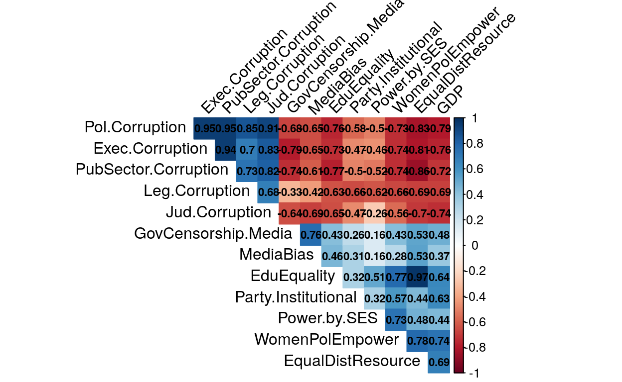
The blue boxes represent a positive correlation between those two variables while the red represents a negative correlation. The saturation of the boxes represent the level of correlation; the more saturated, the higher the correlation. Looking at this plot, it was expected that the four political corruption components (executive, public sector, legislative, and judicial) would be very highly correlated with the overall corruption variable since they make it up. But we can see that the correlation between the overall corruption variable and the judicial variable is lower (0.85) than the others, showing us that there is more variety of legislative corruption among these selected countries. Beyond the corruption variables, all of the other indicators we chose to look at have a negative correlation to overall political corruption of various strength. To see just how much of a relationship these variables had to political corruption we made individual linear regression models to assess.
Show code
c1 <- lm(formula = v2x_corr ~ v2x_execorr, data = vdem_spanish)
#correlation: 0.9455323, adjusted r-squared: 0.8865, p-value: 3.3e-08

c2 <- lm(formula = v2x_corr ~ v2x_pubcorr, data = vdem_spanish)
#correlation: 0.9484681, adjusted r-squared: 0.8924, p-value: 2.257e-08

c3 <- lm(formula = v2x_corr ~ v2lgcrrpt, data = vdem_spanish)
#correlation: 0.8523405, adjusted r-squared: 0.707, p-value: 2.751e-05

c4 <- lm(formula = v2x_corr ~ v2jucorrdc, data = vdem_spanish)
#correlation: 0.9285863, adjusted r-squared: 0.8524, p-value: 2.1e-07

c5 <- lm(formula = v2x_corr ~ v2mebias, data = vdem_spanish)
#correlation: -0.6479888, adjusted r-squared: 0.3785, p-value: 0.006637

c6 <- lm(formula = v2x_corr ~ v2x_gender, data = vdem_spanish)
#correlation: -0.7323050, adjusted r-squared: 0.5031, p-value: 0.001256

c7 <- lm(formula = v2x_corr ~ e_migdppc, data = vdem_spanish)
#correlation: -0.7944973, adjusted r-squared: 0.6049, p-value: 0.0002364

c8 <- lm(formula = v2x_corr ~ v2xeg_eqdr, data = vdem_spanish)
#correlation: -0.8291817, adjusted r-squared: 0.6049, p-value: 0.0002364

c9 <- lm(formula = v2x_corr ~ v2peedueq, data = vdem_spanish)
#correlation: -0.7565669, adjusted r-squared: 0.5419, p-value: 0.0006935

c10 <- lm(formula = v2x_corr ~ e_migdppc, data = vdem_spanish)
#correlation: -0.7944973, adjusted r-squared: 0.6049, p-value: 0.0002364
Unsurprisingly, the political corruption components were very good predictors of overall political corruption (with high adjusted r-squared values and very low p-values). The other indicator variables had various levels of adjusted r-squared values, but were all statistically significant. Wanting to understand the variety of overall corruption scores of this subset of countries, we decided to make a linear regression model of these explanatory variables. To choose which explanatory variables to use, we looked back at the correlation plot to find variables that have high correlation with the overall political corruption variable, but low correlation with each other. This will allow us to capture different but relevant relationships these variables have to political corruption. We ended up choosing these variables to highlight the differences of political corruption in these former Spanish colonies: equal distribution of resources (v2xeg_eqdr), media bias (v2mebias), and GDP per capital (e_migdppc).
Show code
Call:
lm(formula = v2x_corr ~ v2xeg_eqdr + v2mebias + e_migdppc, data = vdem_spanish)

Residuals:
      Min        1Q    Median        3Q       Max
-0.257799 -0.038763 -0.001968  0.038047  0.207234

Coefficients:
              Estimate Std. Error t value Pr(>|t|)
(Intercept)  1.114e+00  7.917e-02  14.069 8.07e-09 ***
v2xeg_eqdr  -3.939e-01  1.777e-01  -2.216   0.0468 *
v2mebias    -1.121e-01  5.412e-02  -2.071   0.0606 .
e_migdppc   -1.864e-05  7.032e-06  -2.650   0.0212 *
---
Signif. codes:  0 '***' 0.001 '**' 0.01 '*' 0.05 '.' 0.1 ' ' 1

Residual standard error: 0.1225 on 12 degrees of freedom
Multiple R-squared:  0.8399,    Adjusted R-squared:  0.7999
F-statistic: 20.98 on 3 and 12 DF,  p-value: 4.587e-05
Show code
#Adjusted R-squared: 0.7999, p-value: 4.587e-05
With a low p-value that represents statistical significance and an adjusted r-squared of almost 0.8, this collection of explanatory variables do a decent job of explaining what makes these countries political corruption scores different. We are not arguing that the higher scores/values of these variables cause higher or lower amounts of political corruption in a country, or that political corruption causes higher or lower scores/values of these variables. We are showing that there is a relationship here. This model shows that higher GDP per capita, less media bias, and a more equal distribution of resources tend to result in less political corruption within this subset of countries. It is also important to note that there might be other variables that explain the differences between these country’s political corruption scores better than the variables we chose, and thus there is more room for research on this phenomenon.
Bibliography
Acemoglu, D., S. Johnson, and J. Robinson. “The Colonial Origins of Comparative Development: An Empirical Investigation.” American Economic Review 91, no. 5 (2001): 1369–1401.
Angeles, Luis, and Kyriakos C. Neanidis. “The Persistent Effect of Colonialism on Corruption.” Economica 82, no. 326 (April 2015): 319–49.
Bulmer-Thomas, V. The Economic History of Latin America since Independence. Cambridge: Cambridge University Press, 2003.
Coatsworth, J. “Inequality, Institutions And Economic Growth in Latin America.” Journal of Latin American Studies 40, no. 3 (2008): 545–69.
Coppedge, Michael, John Gerring, Carl Henrik Knutsen, Staffan I. Lindberg, Jan Teorell, Nazifa Alizada, David Altman, Michael Bernhard, Agnes Cornell, M. Steven Fish, Lisa Gastaldi, Haakon Gjerløw, Adam Glynn, Allen Hicken, Garry Hindle, Nina Ilchenko, Joshua Krusell, Anna Luhrmann, Seraphine F. Maerz, Kyle L. Marquardt, Kelly McMann, Valeriya Mechkova, Juraj Medzihorsky, Pamela Paxton, Daniel Pemstein, Josefine Pernes, Johannes von Römer, Brigitte Seim, Rachel Sigman, Svend-Erik Skaaning, Jeffrey Staton, Aksel Sundström, Ei-tan Tzelgov, Yi-ting Wang, Tore Wig, Steven Wilson and Daniel Ziblatt. 2021. “V-Dem [Country–Year/Country–Date] Dataset v11” Varieties of Democracy Project.
Köbis, Nils C., Daniel Iragorri-Carter, and Christopher Starke. 2018. “A Social Psychological View on the Social Norms of Corruption.” In Corruption and Norms: Why Informal Rules Matter, edited by Ina Kubbe and Annika Engelbert, 31–52. Political Corruption and Governance. Cham: Springer International Publishing.
Sokoloff, K., and S. Engerman. “History Lessons: Institutions, Factors Endowments, and Paths of Development in the New World.” Journal of Economic Perspectives 14, no. 3 (2000): 217–32.
Warf, Barney, and Sheridan Stewart. “Latin American Corruption in Geographic Perspective.” Journal of Latin American Geography 15, no. 1 (2016): 133–55.
Warf, Barney. 2019. Global Corruption from a Geographic Perspective. Vol. 125. GeoJournal Library. Cham: Springer International Publishing.