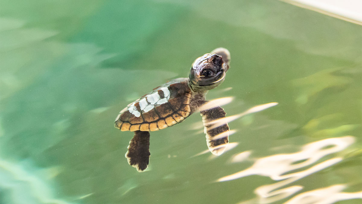
Source: Clearwater Marine Aquarium
The Story
The number of processes, efforts, and relationships that the COVID-19 pandemic has disrupted is endless, from global supply chains for PPE to international mail transport (Manenti et al. 2020). However, a less publicized impact of the lockdowns imposed as a result of COVID-19 involves environmental research. A lot of environmental research relies on remote field stations in isolated and distant places from Moorea in French Polynesia to Antarctica (Ivar do Sul and Costa 2014). With most of the academic research funded in North America and Europe utilizing these field stations for scientific progress, difficult travel arrangements ensues. Journeying to these locations is typically no easy task, with customs, planes, trains, automobiles, and more. However, the COVID-19 pandemic has made travel to these remote field stations very challenging. As a result, many field seasons were canceled as a result of strict in-country restrictions and lockdowns (Rutz et al. 2020). This may mean that in the coming years, 2020 may be a missing puzzle piece in understanding environmental conditions in the context of global climate change.
The Global Biodiversity Information Facility (GBIF) is an international organization committed to increasing the accessibility of biodiversity data. In order to make as much scientific data publicly available as possible, GBIF relies on aggregating records to pool global diversity data for big picture analysis. This often means collecting data from scientific reports, academic journals, human observations directly reported to GBIF and more. Thus, GBIF is a powerful tool but is limited by the ability for data to be collected, reported, and shared.
To better understand how the COVID-19 pandemic may have affected biodiversity research and the ability of scientists and researchers to travel globally, we utilized data from the GBIF API-wrapper package rgbif to answer the following questions:
- How did the COVID-19 pandemic globally impact turtle observations?
- Did the pandemic cause less information on turtle biodiversity data to be submitted to GBIF from 2019 to 2020?
- Are there specific patterns of data collection between countries that differ from 2019 to 2020?
The data
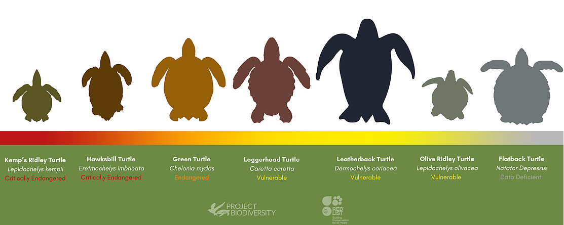
Source: Project Biodiversity
We chose to look at turtle occurrence data from 2019-2020, utilizing the order under which turtles belong (Testudines) to select all turtles (land, aquatic, and marine). Turtle occurrence is a turtle sighting. We chose to look at turtle occurrence because turtles are a highly endangered group of organisms (“The IUCN Red List of Threatened Species” n.d.). For this reason, many organizations and institutions are dedicated to collecting detailed records of turtle occurrence and persistence in the face of climate change (McCrink-Goode 2014). Thus, we surmised that turtles would be a good group of organisms to track potential differences in occurrence data induced by the COVID-19 pandemic.
The wrangling
GBIF mediates an API-wrapper package in R: rgbif. This package allows users to pull occurrence records from the GBIF database using a variety of functions. The occ_data function is the simplest and fastest way to pull occurrence data, as opposed to using more detailed and longer running functions like occ_search.
First we loaded the rgbif package to pull our data, as well as loading any additional packages we needed to data wrangling and visualization
Show code
pacman::p_load(rgbif, tidyverse, rnaturalearth, rnaturalearthdata, rgeo, viridis, ggforce, kableExtra, gridExtra)
Then using the occ_search function in rgbif, we searched for their internal code that calls the Testudines or order for turtles. We use this code to call the Testudines order from now on in our analysis.
Show code
key <- occ_search(scientificName = "Lepidochelys kempii") #order code is 793
Then, to answer our question, we selected to use data only from 2019 and 2020, to compare turtle occurrences pre-COVID-2019 and post-COVID-19 pandemic. The occ_data function does allow for users to call over a series of years. However, we found that in iterating over multiple years, it just splits the total number of occurrences set by the limit argument between the two years, rather than calling that limit for both. When this happened, we didn’t get a spread of data across all 12 months of the year. To achieve gaining data across all 12 months of the year, we ran a separate function for each year and increased the limit to the maximum of 100000.
Show code
turtle_2019<- occ_data(orderKey = 793, year = 2019, limit = 100000)
turtle_2020<- occ_data(orderKey = 793, year = 2020, limit = 100000)
We then transformed these lists into dataframes for each year and selected the following columns:
* species
* iucnRedListCategory
* occurrenceStatus
* year
* month
* day
* eventDate
* collectionCode
* countryCode
* country
* decimalLatitude
* decimalLongitude
* basisOfRecord
We then mutated the eventDate column using the ymd_hms function in the lubridate package.
Show code
turtle_2019_df <- turtle_2019$data %>%
  as.data.frame() %>%
  select(species, iucnRedListCategory, occurrenceStatus, year, month,
         day, eventDate, collectionCode, countryCode, country,
         decimalLatitude, decimalLongitude, basisOfRecord) %>%
  mutate(eventdDate = ymd_hms(eventDate))

turtle_2020_df <-turtle_2020$data %>%
  as.data.frame() %>%
  select(species, iucnRedListCategory, occurrenceStatus, year, month,
         day, eventDate, collectionCode, countryCode, country,
         decimalLatitude, decimalLongitude, basisOfRecord)%>%
  mutate(eventdDate = ymd_hms(eventDate))
We finally bound these two dataframes together into one singular dataframe and wrote it a .csv for a stabler dataset to use the data visualization process. Running the occ_data function takes a really long time to run with the maximum limit number of 100000. Using the .csv allows for a shorter process when working with the data for analysis going forward. From here on, we pull our data from the spreadsheet we have read back in with turtle occurrences from both 2019 and 2020.
Show code
turtle_timeseries <- rbind(turtle_2019_df, turtle_2020_df)
write_csv(turtle_timeseries, "turtle_timeseries.csv")
The results
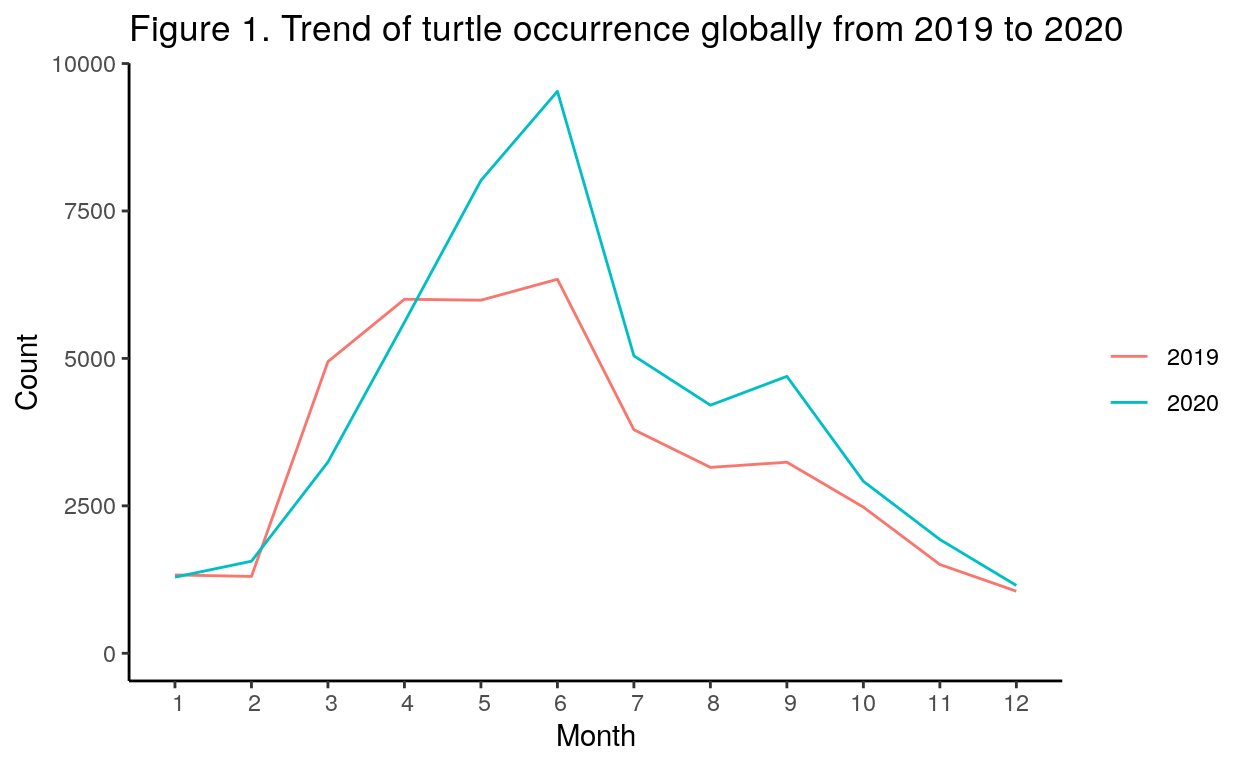
This first figure compares monthly trends of turtle occurrences between 2019 and 2020. We can see here that, surprisingly, more biodiversity data was collected over the course of 2020 than in 2019. The number of turtle occurrences in 2020 started to outnumber the count in 2019 in April and continued this trend. Turtles occurrences were at a peak in June 2020.
Show code
wrangled_turtles %>%
  group_by(month, year) %>%
  count() %>%
  ggplot(mapping =  aes(x = month, y = n, color = factor(year), group = year)) +
  geom_line() +
  scale_x_discrete(limits = c(1, 2, 3, 4, 5, 6, 7, 8, 9, 10, 11, 12)) +
  scale_color_discrete() +
  theme(legend.title = element_blank()) +
  labs(x = "Month",
       y = "Count",
       title = "Figure 1. Trend of turtle occurrence globally from 2019 to 2020")+
  theme_classic() +
  theme(legend.title = element_blank())
To better understand this, we decided to look at how the proportion of turtle occurrences changed between 2019 and 2020. We created a table that compared the turtle occurrences in 10 countries before and after the pandemic. The 10 countries were selected because they reported the most numbers of turtles in 2019, so we were interested in tracking potential turtle occurrence changes in 2020.
Show code
#creating proportion table dataframe to make table figure for top 10 countries
proportion_table <- wrangled_turtles %>%
  filter(countryCode == c("US", "CA", "AU", "MX", "BE", "ZA", "ES", "NL", "GR", "EC")) %>%
  group_by(year, country) %>%
  count() %>%
  pivot_wider(names_from = year, values_from = n) %>%
  mutate(perc_diff = scales::percent((`2020` - `2019`)/sum(`2019`)))%>%
  rename(Country = country, `Percent difference` = perc_diff)
#using kable to make a nice graphic table
proportion_table %>%
  kable(caption = "Proportion of Turtle Occurrences by Countries from 2019 to 2020") %>%
  kable_styling() %>%
  row_spec(which(proportion_table$`2019` > proportion_table$`2020`), background = "pink") %>%
  row_spec(which(proportion_table$`2020` > proportion_table$`2019`), background = "lightgreen") %>%
   add_header_above(c(" ","Turtle Ocurrences" = 2, ""))%>%
  column_spec(1, bold = T) %>%
  footnote(general = "Source: rgbif package, url: https://github.com/ropensci/rgbif",
           number_title = c("Colors"),
           number = c("Red rows represent decreased number of turtle ocurrences from 2019 to 2020",
                      "Green rows represent increased number of turtle occurrences from 2019 to 2020"))
| Country | 2019 | 2020 | Percent difference |
|---|---|---|---|
| Australia | 239 | 98 | -59% |
| Belgium | 61 | 91 | 49% |
| Canada | 395 | 568 | 44% |
| Ecuador | 39 | 25 | -36% |
| Greece | 53 | 22 | -58% |
| Mexico | 80 | 81 | 1% |
| Netherlands | 49 | 20 | -59% |
| South Africa | 66 | 72 | 9% |
| Spain | 63 | 38 | -40% |
| United States of America | 2632 | 3621 | 38% |
| Note: | |||
| Source: rgbif package, url: https://github.com/ropensci/rgbif | |||
| Colors | |||
| 1 Red rows represent decreased number of turtle ocurrences from 2019 to 2020 | |||
| 2 Green rows represent increased number of turtle occurrences from 2019 to 2020 |
According to the table, five countries reported fewer turtle occurrences in 2020 than 2019 and the other five countries reported more turtle occurrences in 2020. However, within each country the magnitude of increase or decrease in turtle occurrence varied widely from a 1% increase in Mexico to a 49% increase in Belgium.
It is worth acknowledging that the total number of turtle occurrences reported by the US is much larger compared to occurrences reported by other countries. As a result, although turtle occurrences decrease for many countries, the US was able to compensate for the decreases reported by other countries. This explains the trends we saw in the first figure. We may need to include observations from other databases/organizations to gain better understanding of how COVID-19 impacted observations during 2020, perhaps non-US affiliated or based groups.
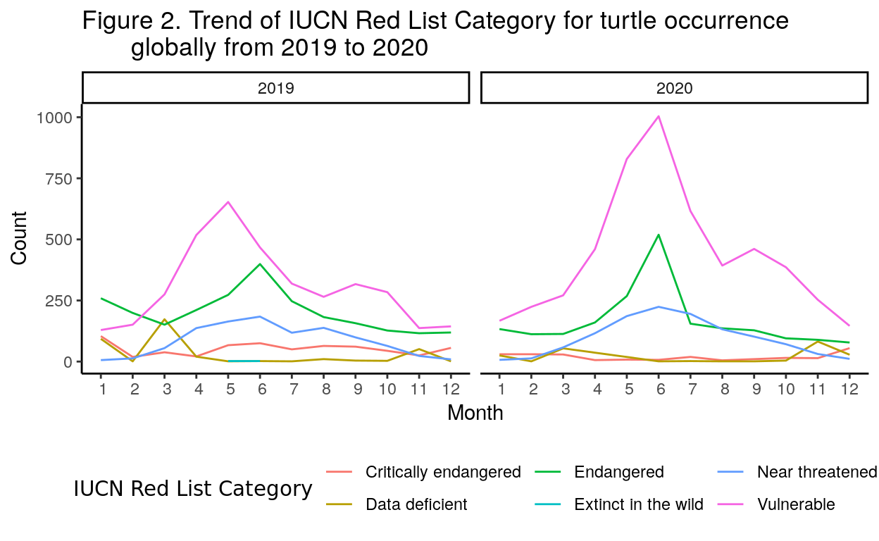
To further understand the differences in turtle occurrences across 2019 and 2020, we were interested in the occurrences based on their IUCN Red List Categories, which code species by their vulnerability in population size and structure.
From our second figure the trends suggest that overall there were just more vulnerable and endangered species identified and reported in 2020 compared to 2019. However, interestingly, there were less critically endangered species and more near threatened species occurrences in 2020 compared to 2019. This may point to more common species being identified and reported, whereas critically endangered species likely reside in very specific regions that may be harder to access and collect data on.
Show code
wrangled_turtles %>%
  drop_na(iucn_labels) %>%
  group_by(month, iucn_labels, year) %>%
  count() %>%
  ggplot(mapping =  aes(x = month, y = n, color = iucn_labels)) +
  geom_line() +
  facet_wrap(~year)+
  scale_x_discrete(limits = c(1, 2, 3, 4, 5, 6, 7, 8, 9, 10, 11, 12)) +
  scale_color_discrete(name = "IUCN Red List Category") +
  theme_classic()+
  theme(legend.position = "bottom",
        legend.title = element_text("IUCN Red List Categories")) +
  labs(x = "Month",
       y = "Count",
       title = "Figure 2. Trend of IUCN Red List Category for turtle occurrence
       globally from 2019 to 2020")
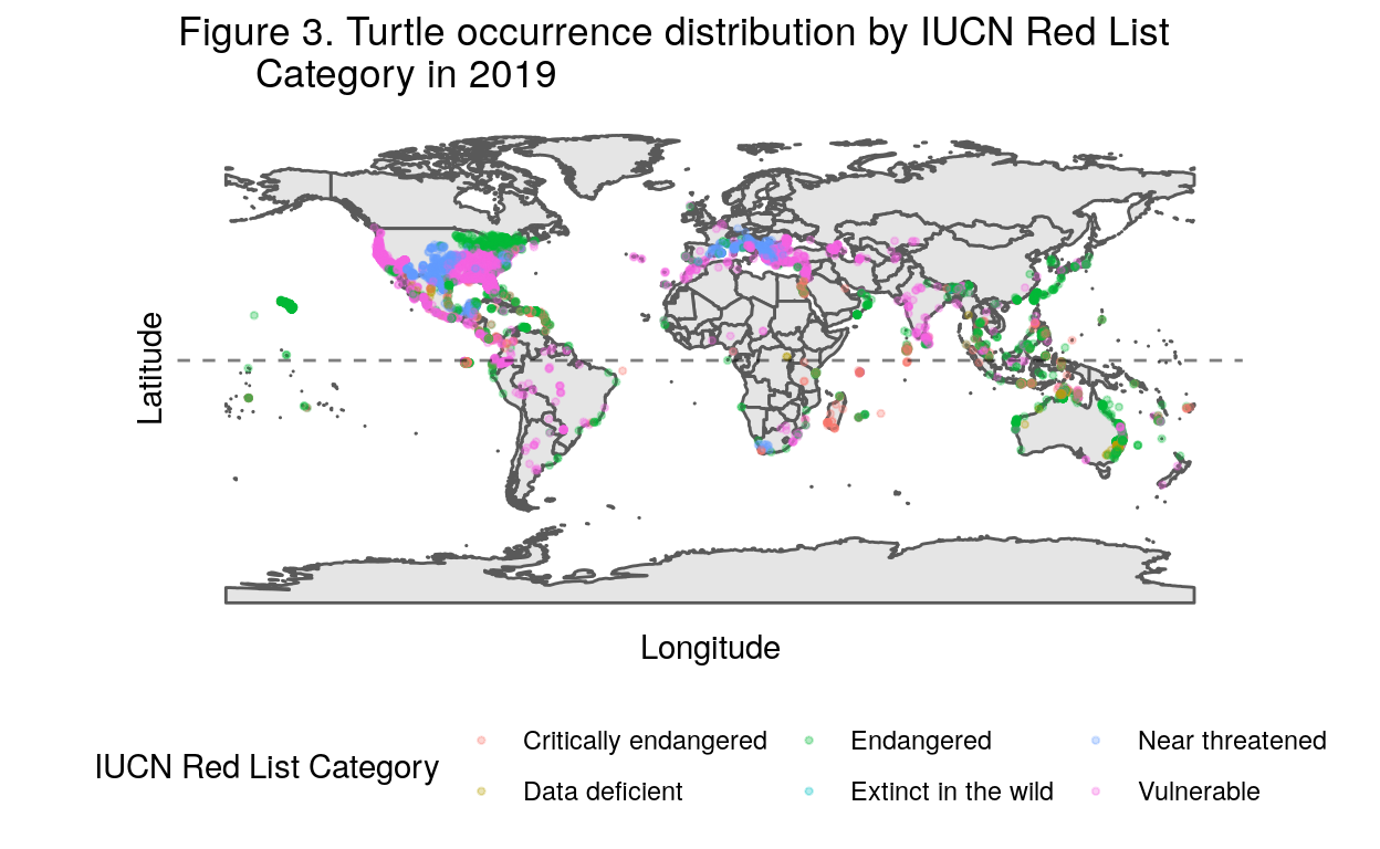
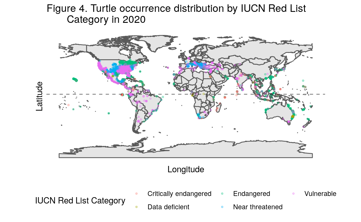
To further examine the changes in turtle occurrence, we plotted the locations of the reported turtles by their IUCN Red List Category onto a global map. Consistent with the last plot, there was a small increase in vulnerable and endangered species reported by the US but not by other countries in 2020. But the overall global trend of turtle species distribution in places where biodiversity is studied does not seem to vary much inter-annually.
Show code
#plotting up occurrence data in a map ~~~ 2019
ggplot(data = world) +
  geom_sf() +
  geom_point(data =  wrangled_turtles %>%
  drop_na(iucn_labels) %>%
    filter(year == "2019"),
             aes(x = decimalLongitude, y = decimalLatitude, color = iucn_labels),
             size = 0.8, alpha = 0.3) +
  geom_hline(yintercept = 0, alpha = 0.5, linetype = "dashed") +
  theme_classic() +
  theme(legend.position = "bottom") +
  scale_color_discrete(name = "IUCN Red List Category") +
  ylab("Latitude") +
  xlab("Longitude") +
  labs(title = "Figure 3. Turtle occurrence distribution by IUCN Red List
       Category in 2019")
Show code
#plotting up occurrence data in a map ~~~ 2020
ggplot(data = world) +
  geom_sf() +
  geom_point(data = wrangled_turtles %>%
  drop_na(iucn_labels) %>%
    filter(year == "2020"),
             aes(x = decimalLongitude, y = decimalLatitude, color = iucn_labels),
             size = 0.8, alpha = 0.3) +
  geom_hline(yintercept = 0, alpha = 0.5, linetype = "dashed") +
  theme_classic() +
  theme(legend.position = "bottom") +
  scale_color_discrete(name = "IUCN Red List Category") +
  guides(color = guide_legend(nrow = 2)) +
  ylab("Latitude") +
  xlab("Longitude") +
  labs(title = "Figure 4. Turtle occurrence distribution by IUCN Red List
       Category in 2020")
It is difficult to conclude how COVID-19 impacted turtle observations without incorporating more data from other databases or directly surveying the scientists who collect observations. The data included in the GBIF database is confounded by many factors, involving scientists, their country of origin, and their economic status. Our exploration determined that overall turtle observations did not decrease in 2020 but some countries contributed less observations than in the 2019 year. However, further examination is required to rigorously conclude how and if turtle occurrences were significantly impacted by the COVID-19 pandemic.
Ivar do Sul, Juliana A., and Monica F. Costa. 2014. “The Present and Future of Microplastic Pollution in the Marine Environment.” Environmental Pollution (Barking, Essex: 1987) 185 (February): 352–64. https://doi.org/10.1016/j.envpol.2013.10.036.
Manenti, Raoul, Emiliano Mori, Viola Di Canio, Silvia Mercurio, Marco Picone, Mario Caffi, Mattia Brambilla, Gentile Francesco Ficetola, and Diego Rubolini. 2020. “The Good, the Bad and the Ugly of COVID-19 Lockdown Effects on Wildlife Conservation: Insights from the First European Locked down Country.” Biological Conservation 249 (September): 108728. https://doi.org/10.1016/j.biocon.2020.108728.
McCrink-Goode, Melissa. 2014. “Pollution: A Global Threat.” Environment International 68 (July): 162–70. https://doi.org/10.1016/j.envint.2014.03.023.
Rutz, Christian, Matthias-Claudio Loretto, Amanda E. Bates, Sarah C. Davidson, Carlos M. Duarte, Walter Jetz, Mark Johnson, et al. 2020. “COVID-19 Lockdown Allows Researchers to Quantify the Effects of Human Activity on Wildlife.” Nature Ecology & Evolution 4 (9): 1156–9. https://doi.org/10.1038/s41559-020-1237-z.