New York City Uber Data
Back in 2014 and 2015, New York City was complaining about Uber displacing their iconic taxi cars. At the time, Uber hadn’t released any of its data so there was no real way to easily evaluate these claims. But through a Freedom of Information Law request, Uber’s data on pickups in NYC was made publicly available. Focusing in on May of 2015 as a case study, let’s take a look at New York City’s Uber usage. Our main focus will revolve around how Uber is impacting the city’s traffic, and if it actually represents a significant source of city transportation.
Data Acquisition and Wrangling
First, we found a compiled file of dates, times, dispatching bases, and locations describing every logged ride that someone took in an Uber in May.
To better understand the distribution of rides across various time scales like hour, week, and day we created new columns in the dataset that contained this information by converting the date/time stamp into easy-to-parse formats. These new variables described the hour the ride was taken, the day of the week, and the minute of pickup.
# Reformat and add date and time variables of uber dataset
library(lubridate)
uber <- uber %>%
  mutate(Pickup_date = mdy_hm(Pickup_date)) %>%
  mutate(Day = factor(day(Pickup_date)),
         Month = factor(month(Pickup_date, label = TRUE)),
         Year = factor(year(Pickup_date)),
         DayOfWeek = factor(wday(Pickup_date, label = TRUE)),
         Hour = factor(hour(Pickup_date)),
         Minute = factor(minute(Pickup_date)))
For additional context and because a number is not a very human readable representation of a location, we used supplemental datasets to add both the dispatching base name and the names of the boroughs and zones where the customer was picked up.
Show code
# Read in file of base codes and their corresponding names
bases <- read_csv(here("_posts/2021-03-07-new-york-city-uber-rides/data/uber_base_codes.csv"))

# Join bases to uber to get names of dispatch bases
uber <- left_join(uber, bases, by = c("Dispatching_base_num" = "BaseCode"))

# Read in location data (ID, zone, borough)
location <- read_csv(here("_posts/2021-03-07-new-york-city-uber-rides/data/taxi_zone_lookup.csv"))

# Join location data to uber by location ID
uber <- left_join(uber, location, by = c("locationID" = "LocationID"))
Visualizing Uber Ridership Patterns
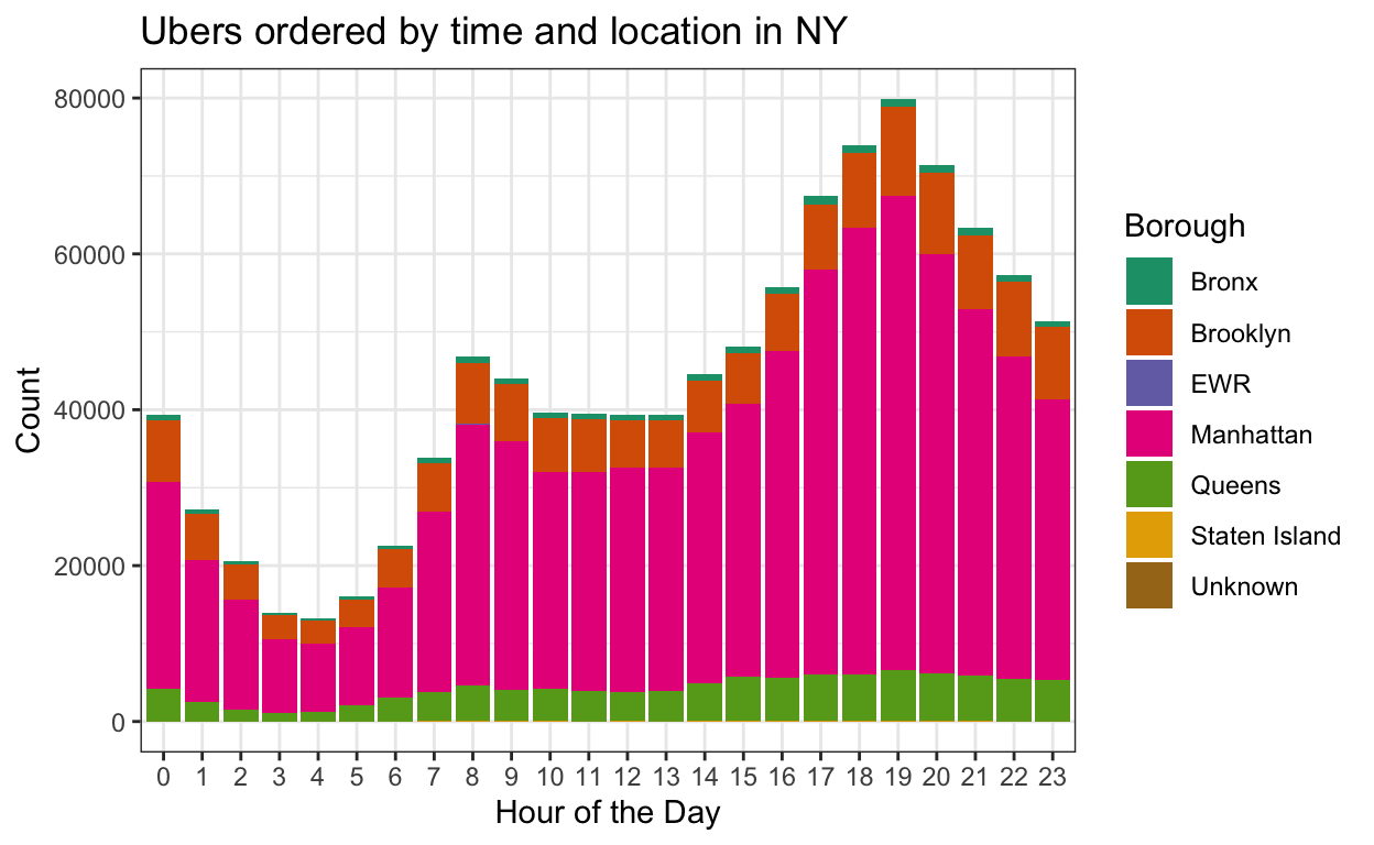
First, we needed to explore what ridership looks like during May 2015. We did this by graphing the number of rides recorded over both hour of the day and day of the week and observing the borough that the Uber pickup occurred in. Over the hours in the day, it seems that rides are peaking in the evening between 5 to 9 pm with the most rides observed at 7 pm. Maybe some of this ridership is coming from commuters but if that were true, we would also expect to see a morning peak that was comparable in magnitude which we don’t observe.
Show code
# Bar chart by hour and borough
ggplot(data = uber, mapping = aes(x = Hour, fill = Borough)) +
  geom_bar() +
  scale_fill_brewer(type = "qual", palette = "Dark2") +
  labs(title = "Ubers ordered by time and location in NY", x = "Hour of the Day", y = "Count") +
  theme_bw()
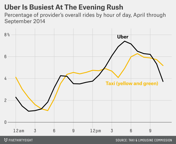
Because we are good data scientists, we questioned whether this particular month is a reasonable snapshot of the larger trends in ridership. Luckily, FiveThirtyEight produced a plot of ridership percentage over the hours in a day for all Uber rides that took place April to September in 2014. They produced the following graphic using much more ridership data and we can see that, all in all, this month does essentially replicate the trends that they observe over the hours in a day.
The most served borough is Manhattan, which is unsurprising given its one of the densest places on earth population-wise and also a major tourist attraction.
What might be surprising is that Wednesday was the busiest day of the week for Uber rides, at least for May of 2015. We expected that more people would order Ubers on the weekends or a Friday night to go out, but weekdays were often just as, if not more busy for Uber rides. Manhattan takes the cake again for the most popular borough ordering Ubers on any day of the week, though.
Show code
# bar plot by weekday
ggplot(data = uber, mapping = aes(x = DayOfWeek, fill = Borough)) +
  geom_bar() +
  scale_fill_brewer(type = "qual", palette = "Dark2") +
  labs(title = "Ubers ordered by day of week and location in NY", x = "Day", y = "Count") +
  theme_bw()
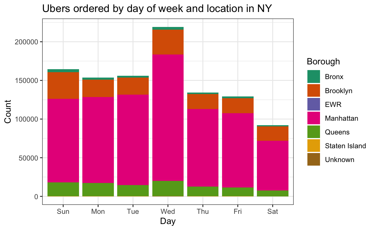
Perhaps I am just a naive non-New-Yorker, but here I was, thinking Queens or Brooklyn would have just as many Ubers ordered as Manhattan. Brooklyn is 3 times the size of Manahttan and Queens is 5 times the size of it, and yet, if we look at the number of Uber rides even on any given weekday, Brooklyn falls short, at least compared to Manhattan. The values in the table show how many Ubers were ordered per Borough on a given day of the week, with the total adding to 1. On a Saturday night, Manhattan had .703, which makes up the majority out of all the Boroughs! Brooklyn only made up .201 and Queens had even less at .081. While yes, there are Boroughs with far fewer Ubers ordered than either Brooklyn or Queens, the size of the two makes you wonder if $ is responsible for the mismatched sizes of Boroughs and number of Ubers ordered.
Show code
library(gt)

#wrangling table
uber_table <- uber %>%
  group_by(DayOfWeek) %>%
  count(Borough) %>%
    mutate(p = n/sum(n)) %>%
  select(-c(n)) %>%
  pivot_wider(names_from = DayOfWeek, values_from = p)

uber_table$Fri[is.na(uber_table$Fri)] <- 0

#gt table for proportions
uber_table %>%
  gt() %>%
  fmt_number(columns = vars("Sun", "Mon", "Tue", "Wed", "Thu", "Fri", "Sat"), decimals = 3) %>%
  tab_header(
    title = md("Proportion of Ubers Ordered in a Borough Each Day"))  %>%
  tab_style(
    style = list(
      cell_fill(color = "lightcyan")),
    locations = cells_body(
      columns = vars("Sun", "Mon", "Tue", "Wed", "Thu", "Fri", "Sat"),
      rows = Borough == "Manhattan"
    )) %>%
  tab_style(
    style = list(
      cell_fill(color = "lightgoldenrod")),
    locations = cells_body(
      columns = vars("Sun", "Mon", "Tue", "Wed", "Thu", "Fri", "Sat"),
      rows = Borough == "Queens"
    )) %>%
   tab_style(
    style = list(
      cell_fill(color = "lightpink")),
    locations = cells_body(
      columns = vars("Sun", "Mon", "Tue", "Wed", "Thu", "Fri", "Sat"),
      rows = Borough == "Brooklyn"
    )) %>%

  #source footnote
  tab_source_note(source_note = "From: https://github.com/fivethirtyeight/uber-tlc-foil-response/blob/master/uber-trip-data/uber-raw-data-janjune-15") %>%

  #footnote about rounding table values
tab_footnote(footnote = "All proportions in table were rounded to three decimal places.",
               locations = cells_title())
| Proportion of Ubers Ordered in a Borough Each Day1 | |||||||
|---|---|---|---|---|---|---|---|
| Borough | Sun | Mon | Tue | Wed | Thu | Fri | Sat |
| Bronx | 0.023 | 0.016 | 0.015 | 0.016 | 0.015 | 0.017 | 0.014 |
| Brooklyn | 0.209 | 0.147 | 0.142 | 0.146 | 0.145 | 0.151 | 0.201 |
| EWR | 0.000 | 0.000 | 0.000 | 0.000 | 0.000 | 0.000 | 0.000 |
| Manhattan | 0.658 | 0.723 | 0.750 | 0.747 | 0.747 | 0.742 | 0.703 |
| Queens | 0.110 | 0.113 | 0.092 | 0.090 | 0.092 | 0.089 | 0.081 |
| Staten Island | 0.000 | 0.000 | 0.000 | 0.000 | 0.001 | 0.001 | 0.001 |
| Unknown | 0.000 | 0.000 | 0.000 | 0.000 | 0.000 | 0.000 | 0.001 |
| From: https://github.com/fivethirtyeight/uber-tlc-foil-response/blob/master/uber-trip-data/uber-raw-data-janjune-15 | |||||||
|
1
All proportions in table were rounded to three decimal places.
|
|||||||
Concluding Thoughts
While taxis have long been hailed throughout New York, the times are changing and ride shares like Uber are becoming more and more popular. In fact, Uber usage overtook yellow cab usage in 2017. The increasing use of cell phones make using Uber a common pick, since it functions through an app and doesn’t require cash or card payment. And, of course, it has become trendy. However, the largest Boroughs in New York don’t seem to be indulging in Uber rides to the same extent as Manhattan, where the most Ubers were ordered on any day of the week. It doesn’t look like taxis will be phased out any time soon in most Boroughs throughout New York, expect maybe in Manhattan, where even in the middle of the work week, Ubers were being ordered out the wazoo.
As to our question of how New York City is being impacted by Uber, this story shows that Ubers are becoming part of the everyday transportation in the city. Of course, there are still millions of commuters, tourists, and traveling New Yorkers who make use of taxis and public transit1, but looking at the sheer volume of pickups that happen in Manhattan, one of the most congested areas of New York, there’s no doubt that the Uber is impacting the landscape of the city’s transportation.
43 million pickups by cabs in 2015; 1.72 billion subway riders in 2015↩