Introduction
The collective programming experience of the students of this Data Science class is quite diverse. Some people just took intro stats the previous semester, while others have been coding since their freshman year of high school. Some only know R, some have a couple of other coding languages up their sleeve. This wide range of programming experience and knowledge is similarly reflected in the Kaggle community. Kaggle is an online community of data scientists and machine learning practitioners established to attract, nurture, train, and challenge members to solve data science, machine learning, and predictive analytics problems.
Within the Kaggle community, members/users have different education backgrounds, programming experience, and program language preferences. Noting the vastly diverse background of programmers, we became interested in how these components relate to one another. Since 2017, Kaggle has been surveying its users to break down trends within their community of data scientists. This survey captures how key demographics relate to education levels and usage of various programming languages.
Using their 2020 survey data, we attempted to create two models to predict different trends in the Kaggle community. Specifically, we ask, can we predict (1) the highest education of programmers and (2) whether a user will be python-dominant or R-dominant by the number of years a respondent has been coding and the number of coding languages known by a user?
About: the data
The original data set had 20,036 observations and 355 variables. We narrowed it down to 19 variables that pertain to our main research questions. There were 13 choices for the survey question ‘What programming languages do you use on a regular basis?’, which consisted of one ‘other’ option, one ‘none’ option, and 12 programming languages. We also included the demographic info about age, the highest level of education, current role/recent title if retired, and the number of years programming. We then built a composite variable, the language index (lang_index) which reflects the sum of all known languages for each respondent.
We then created another 3 variables that refer to users preference of R vs. python. The first two (python_no_rand r_no_python) refer to Kaggle users that use either R or python programming, but not the other. The third variable (rp_flag) flags the survey respondents preference of python or R. A python-dominant user is defined as someone who uses python daily but does not use R. Conversely, an R-dominant user uses R on a daily basis but does not use python. Restricting the data set to look at the Kaggle survey respondents that uses either R or python (not both), the number of observations/applicable respondents in this new data frame decreased to 12,763.
About: our models
We use a multinomial logistic regression using the multinom function from the nnet package to estimate two multinomial logistic regression models. We chose multinom over other packages because many, for example, mlogit, require lots of data reshaping. Multinom supports some nice regression summaries, but we need to calculate the p scores manually and exponentiated coefficients to use as risk ratios. We use this model because it is a model that can be used to predict probabilities of outcomes for categorical dependent variables, based on a set of independent variables.
In both models, years_programming and the number of languages used daily (language index) are the independent variables. The level of education of a user (model 1) and the preferred programming language, R vs. python, (model 2) are our dependent variables. Just reiterate, our models use those independent variables to predict the dependent variable.
Can we predict education of Kaggle users?
Preliminary exploration
We first subset the data to look at how one’s education relates to the number of years a person has spent programming.
Show code
x <- c("I have never written code", "< 1 years", "1-2 years", "3-5 years", "5-10 years", "10-20 years",
       "20+ years")

yr_edu_count1 <- as.data.frame(with(df, table(years_programming, highest_edu)))

yr_edu_count <- pivot_wider(yr_edu_count1, names_from = highest_edu, values_from = Freq)

col_order <- c("years_programming", "No formal education past high school", "Professional degree",
               "Some college/university study without earning a bachelor’s degree", "Bachelor’s degree",
               "Master’s degree", "Doctoral degree", "I prefer not to answer")

yr_edu_count <- yr_edu_count[, col_order] %>%
  arrange(sapply(years_programming, function(y) which(y == x)))

kable(yr_edu_count, caption = "Frequency of Years Programming by Education") %>%
  kable_styling(bootstrap_options = c("striped", "condensed", "responsive")) %>%
  column_spec(2, color = "white",
              background = spec_color(yr_edu_count$'No formal education past high school'[1:7], end = 0.7)) %>%
  column_spec(3, color = "white",
              background = spec_color(yr_edu_count$'Professional degree'[1:7], end = 0.7)) %>%
  column_spec(4, color = "white",
              background = spec_color(
                yr_edu_count$'Some college/university study without earning a bachelor’s degree'[1:7],
                end = 0.7)) %>%
  column_spec(5, color = "white",
              background = spec_color(yr_edu_count$'Bachelor’s degree'[1:7], end = 0.7))%>%
  column_spec(6, color = "white",
              background = spec_color(yr_edu_count$'Master’s degree'[1:7], end = 0.7)) %>%
  column_spec(7, color = "white",
              background = spec_color(yr_edu_count$'Doctoral degree'[1:7], end = 0.7))
| years_programming | No formal education past high school | Professional degree | Some college/university study without earning a bachelor’s degree | Bachelor’s degree | Master’s degree | Doctoral degree | I prefer not to answer |
|---|---|---|---|---|---|---|---|
| I have never written code | 36 | 77 | 101 | 407 | 377 | 79 | 47 |
| < 1 years | 52 | 131 | 280 | 1442 | 1155 | 167 | 86 |
| 1-2 years | 53 | 125 | 293 | 2101 | 1627 | 220 | 86 |
| 3-5 years | 29 | 115 | 188 | 1723 | 2031 | 397 | 63 |
| 5-10 years | 14 | 81 | 87 | 603 | 1233 | 504 | 30 |
| 10-20 years | 17 | 92 | 49 | 325 | 753 | 492 | 23 |
| 20+ years | 24 | 59 | 62 | 218 | 529 | 407 | 30 |
This table visually highlights a trend that the more education a Kaggle community member has, the more likely it is that they have spent many, many years programming. For example, most of the respondents with doctoral degrees are placed in the latter three categories of year_programming (5-10 years, 10-20 years, and 20+ years). However, the respondents with (1) no formal education past high school, with (2) a professional degree, and with (3) some college/university study without earning a bachelor’s degree have similar patterns with most of those respondents have less than 1 year or 1-2 years of coding/programming experience.
Now to visualizing how education relations to the number of programs a respondents knows.
Show code
mean_sd_plot <- ggplot(df, aes(x = lang_index, y = highest_edu)) +
  geom_jitter(alpha = 0.07) +
  stat_summary(fun.data = mean_sdl, fun.args = list(mult=1),
                 geom="pointrange", color="red") +
  theme_bw() +
  labs(x = "Number of Programming Languages Known by Respondent", y = "Highest Education of Respondent",
       title = "The Number of Programming Languages Known by\nEach Respondent, Grouped by Education Level\n(Kaggle Survey Respondents 2020)",
       subtitle = "The means and standard deviations are in red.")+
  scale_y_discrete(limits = rev(c("No formal education past high school", "Professional degree",
               "Some college/university study without earning a bachelor’s degree", "Bachelor’s degree",
               "Master’s degree", "Doctoral degree", "I prefer not to answer")),
               labels = function(x) str_wrap(x, width = 25)) +
  geom_label(stat = 'summary', fun.data = mean_sdl, aes(label = round(..x.., 2)), nudge_y = 0.2, hjust = 0,
            color = "red", size = 2) +
  scale_x_continuous(breaks = c(0,1,2,3,4,5,6,7,8,9,10,11,12))
mean_sd_plot
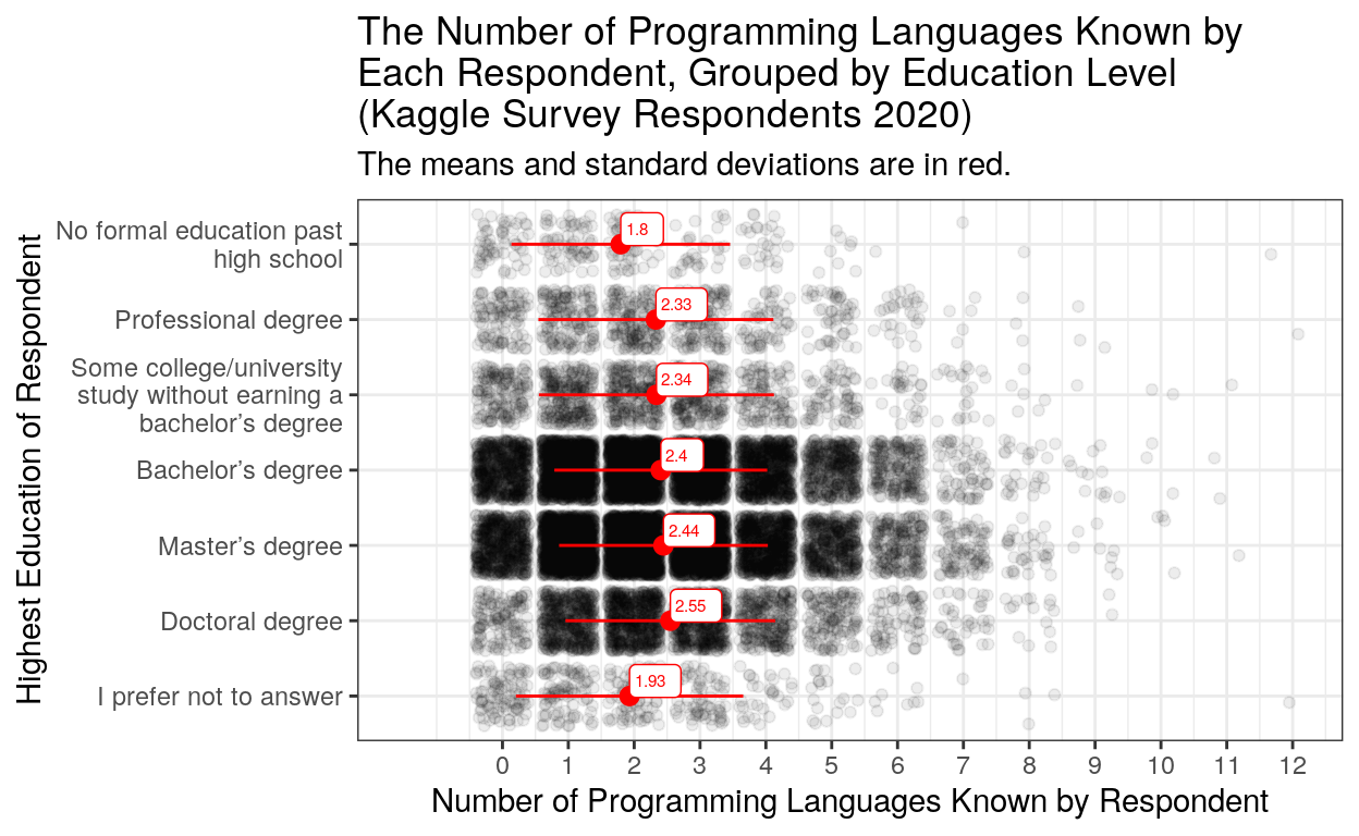
This plot shows the mean and standard deviation of the number of programming languages known by each education grouping. There seems to be a slight increase of number languages known as the amount of education one has increases (the mean of Kaggle members with no formal education past high school is 1.76 while the mean of Kaggle members with a doctoral degree is 2.55). This visualization shows that that the number of programming languages a Kaggle user knows is slightly related to their education.
Model to Predict Kaggle User Education Levels
Looking at those two visualizations, we hypothesize that our model with predict that the more time a user has spent coding (years_programming) and the more languages they know (lang_index), the higher the odds are that that user has a higher education.
To predict Kaggle user education levels, we chose the “No formal education past high school” option within the highest_edu variable and “< 1 years” option within the years_rogramming variable to be the baseline for the model. The outputs of the model is calculated relative to these two options and thus are not included in the tables. Meaning, changing the baseline for the models would not change the results of the model but would change what the results are relative to.
The first thing to note about the model is the residual deviance and AIC look high. This model has a residual deviance of 50938.39 and an AIC of 51034.39. The residual deviance tells us us how well our response is predicted by the model when the predictors are included. The Akaike information criterion (AIC) is an estimator of prediction error which is also used in model selection like residual deviance to help us select which model fits the data best. With AIC lower is better, since it indicates a better fit, but in most cases it is used to choose between model calibration, so it is not of much importance to our analysis.
Now looking at the p-value output from this model. The p-value gives us evidence against our null hypothesis, said differently it tells us if it is likely our model is predicting something other than noise.
Show code
kable(p_m1, caption="P Values") %>%
  kable_styling(bootstrap_options = c("striped", "hover", "condensed", "responsive"))
| highest_edu | (Intercept) | 0 years | 1-2 years | 3-5 years | 5-10 years | 10-20 years | 20+ years | lang_index |
|---|---|---|---|---|---|---|---|---|
| Professional degree | 0.0016615 | 0.6151550 | 0.5272782 | 0.2530987 | 0.0494757 | 0.0824614 | 0.3864851 | 0.0066832 |
| Some college/university study without earning a bachelor’s degree | 0.0000000 | 0.4140206 | 0.6766418 | 0.9312211 | 0.7719995 | 0.0047484 | 0.0002631 | 0.0000984 |
| Bachelor’s degree | 0.0000000 | 0.0278996 | 0.1919339 | 0.0135626 | 0.4345033 | 0.0345921 | 0.0000002 | 0.0005035 |
| Master’s degree | 0.0000000 | 0.0299650 | 0.1874566 | 0.0000126 | 0.0000458 | 0.0636445 | 0.4959609 | 0.0283128 |
| Doctoral degree | 0.0000000 | 0.2640676 | 0.2864083 | 0.0000000 | 0.0000000 | 0.0000000 | 0.0000000 | 0.4607899 |
| I prefer not to answer | 0.0994836 | 0.7844630 | 0.8097927 | 0.4901060 | 0.6391202 | 0.4152618 | 0.2399397 | 0.2100756 |
We find that there is a mixed bag of p-values here. There are not any columns or rows with completely significant values. Notably, in the language index, the p-values for a doctoral degree and master’s degree are insignificant.
Now looking at the risk ratios calculated form the predictive model. The risk ratios we calculate are obtained by exponentiating the coefficients from our logistic regression and can be interpreted as a multiplier for the likelihood that the outcome occurs. For example, if the baseline is high school education, and someone with a masters has a risk ratio 2 in their coding for 10 years variable, then we can say those who have been coding for 10 years are twice as likely to have a masters than those who are only high school educated.
Show code
kable(risk_m1, caption="Risk Ratios") %>%
  kable_styling(bootstrap_options = c("striped", "hover", "condensed", "responsive"))
| highest_edu | (Intercept) | 0 years | 1-2 years | 3-5 years | 5-10 years | 10-20 years | 20+ years | lang_index |
|---|---|---|---|---|---|---|---|---|
| Professional degree | 1.856594 | 1.1522673 | 0.8626877 | 1.3608870 | 1.9420637 | 1.7417239 | 0.7684061 | 1.184508 |
| Some college/university study without earning a bachelor’s degree | 3.491366 | 0.8038050 | 0.9145242 | 0.9782199 | 0.9087483 | 0.3965772 | 0.3402199 | 1.263975 |
| Bachelor’s degree | 19.339892 | 0.5847299 | 1.2980153 | 1.8035402 | 1.2736616 | 0.5376648 | 0.2465988 | 1.218627 |
| Master’s degree | 17.814776 | 0.5879868 | 1.3027043 | 2.8397560 | 3.5137987 | 1.7147825 | 0.8361962 | 1.132487 |
| Doctoral degree | 2.982897 | 0.7358273 | 1.2671367 | 4.1177382 | 10.7678683 | 8.5734482 | 4.9909888 | 1.043805 |
| I prefer not to answer | 1.420410 | 0.9193816 | 0.9416501 | 1.2220872 | 1.1917441 | 0.7373046 | 0.6720036 | 1.090963 |
Across programming experience, trends also matched our expectations with those with more experience predicting education level. We were surprised by the lack of variation in the magnitude of risk ratios for several languages known since one would assume you learn more languages as you progress higher into academia. But this might be expected since there was lots of heterogeneity in significance levels for the language index, possibly due to multicollinearity issues during index construction.
Can we predict whether a Kaggle user will be python-dominant or R-dominant?
Preliminary exploration
A python-dominant user is defined as someone who uses python daily but does not use or know R. Conversely, an R-dominant user uses R on a daily basis but does not use or know python.
Show code
ggplot(pie_chart, aes(x = "", y = Freq, fill = Var1)) +
  geom_bar(stat = "identity", width = 1) +
  coord_polar("y", start = 0) +
  geom_text(aes(label = percentage), color = "white")+
  scale_fill_brewer(palette="Dark2") +
  theme_void() +
  labs(fill = "Programming Language",
       title = "Comparing the number of Python users vs R users",
       subtitle = "This reflects Kaggle users that know/use either python or R, but not both.")
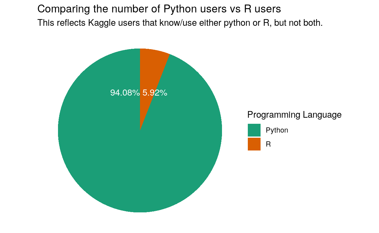
This pie chart shows us that the subset of the original survey data of users who no either R or python, but not both, is made up of mostly python users and very few R users. This is important information for rest of our plots an out predictive model.
Now, to visualizing the mean and standard deviations of number programming languages known users were are #teampython and #teamR.
Show code
mean_sd_plot2 <- ggplot(python_vs_r_df, aes(x = lang_index, y = rp_flag)) +
  geom_jitter(alpha = 0.07) +
  stat_summary(fun.data = mean_sdl, fun.args = list(mult=1),
                 geom="pointrange", color="red") +
  theme_bw() +
  labs(x = "Number of Programming Languages Known by Respondent", y = "Preferred Programming Language",
       title = "The Number of Programming Languages Known by\nEach Respondent, Grouped by their Language Preverence\n(Kaggle Survey Respondents 2020)",
       subtitle = "The means and standard deviations are in red.")+
  scale_y_discrete(labels = function(x) str_wrap(x, width = 25)) +
  geom_label(stat = 'summary', fun.data = mean_sdl, aes(label = round(..x.., 2)), nudge_y = 0.2, hjust = 0,
            color = "red", size = 2) +
  scale_x_continuous(breaks = c(0,1,2,3,4,5,6,7,8,9,10,11,12))
mean_sd_plot2
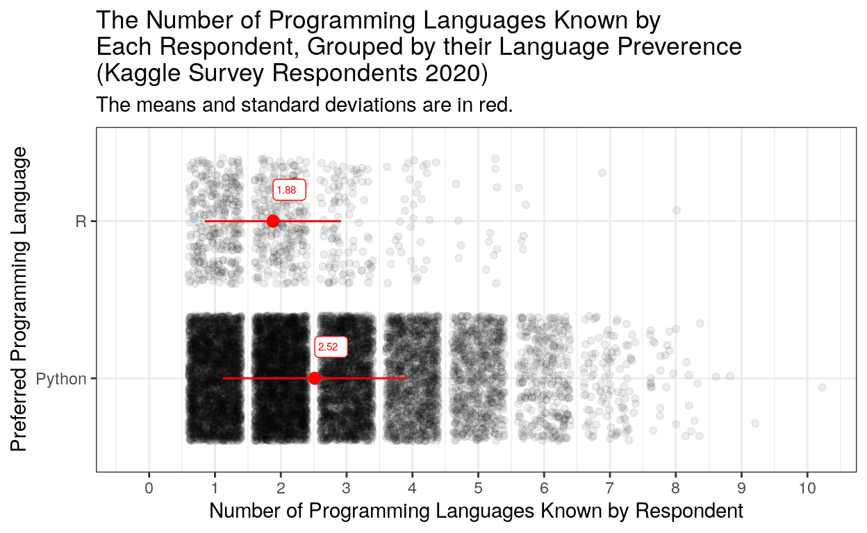
This plot shows that python users in this subset of the data, on average, know more languages than R users (2.52 mean vs. 1.88 mean).
Now, to how years spent prgraming relates to R and python users.
Show code
kable(yr_rvp_count, caption = "Frequency of Years Programming by Preferred programming Language/n(R vs. Python)") %>%
  kable_styling(bootstrap_options = c("striped", "condensed", "responsive")) %>%
  column_spec(2, color = "white",
              background = spec_color(yr_rvp_count$'Python'[1:7], end = 0.7)) %>%
  column_spec(3, color = "white",
              background = spec_color(yr_rvp_count$'R'[1:7], end = 0.7))
| years_programming | Python | R |
|---|---|---|
| < 1 years | 2286 | 122 |
| 1-2 years | 3176 | 163 |
| 3-5 years | 3101 | 181 |
| 5-10 years | 1632 | 124 |
| 10-20 years | 1062 | 82 |
| 20+ years | 751 | 83 |
This table does not show a clear trend. Meaning, it is unclear whether years_programming is directly related enough to the preferred programming language. This could be due to the way we subset our data. We ignored respondents that knew both R and python in order to highlight differences in the users, but it is possible that it is common for R users to know python or for python users to know R. It is impossible to say based off of the Kaggle survey data.
The Model to Predict Kaggle User Language Preference (R vs. Python)
In this model, R is the baseline, so all ratios are relative to R users as it is the control. Since the model is multivariate, the difference in outputs will be read inversely. Our preliminary findings did not look so good, but we hypothesize that users that know more programming languages are likely to be python users. We make this conclusion because there is a clear relationship between number of programming languages known by a respondent and their preferred programming language.
Again the residual deviance and AIC is high(Residual Deviance: 5455.523; AIC: 5469.523), in fact, higher than the first model, indicating this is a less helpful model fit for our data.
Show code
kable(p_m2, caption = "P-Values")%>%
  kable_styling(bootstrap_options = c("striped", "hover", "condensed", "responsive"))
| variable | p-value |
|---|---|
| (Intercept) | 0.0000000 |
| 1-2 years | 0.1632334 |
| 3-5 years | 0.0001684 |
| 5-10 years | 0.0000000 |
| 10-20 years | 0.0000000 |
| 20+ years | 0.0000000 |
| lang_index | 0.0000000 |
All variables are significant at the .001 level with the exception of the cohort that has been programming for 1-2 years.
Show code
kable(risk_m2, caption="Risk Ratios")%>%
  kable_styling(bootstrap_options = c("striped", "hover", "condensed", "responsive"))
| variable | coef_2 |
|---|---|
| (Intercept) | 8.0405991 |
| 1-2 years | 0.8412879 |
| 3-5 years | 0.6299602 |
| 5-10 years | 0.4580970 |
| 10-20 years | 0.4112353 |
| 20+ years | 0.2610126 |
| lang_index | 1.7062531 |
The above shows the risk ratios for the different variables relative to R as the baseline. We see that across the board, ignoring the insignificant 1-2 years, being a python user makes you less than 3/4 as likely to have been programming for longer across all the experience cohorts. Interestingly, exclusive python users are likely to know 1.7 as many languages, suggesting there might be something about it that makes it a great integration multipurpose language versus R, which seems to be a legacy academia and enterprise tool at this point in time. Even though the cohort of least experienced programmers are still more likely to be R users, it is by far the area for which R’s user penetration may be struggling. It was particularly surprising that python users had a 25% chance of having programmed for 20+ years. Maybe this indicates a degree of path dependency in R when it comes to ecosystems and frameworks.
Conclusion
The model (model 1) predicting education level was not a great fit, lots of insignificance which makes sense since there’s so much stuff that goes into determining something like education
The python vs R model showed how dominant R was for experienced users, and had more significant results across the board. However python users tended to know more languages which makes sense since it has a broader use case then R and is not proprietary in any shape or form.