The process of hybridization refers to interbreeding between populations that are distinct genetically due to ecological or reproductive isolation Grant, 1981. Ecological isolation refers to populations separated by distance, and reproductive isolation refers to populations that have developed different reproductive methods such as distinct pollinators. Hybridization is thought to be a common process involved in vascular plant evolution, especially for certain genera and families Ellstrand et al., 1996.
Oak hybridization in particular has a vast amount of research regarding hybridization rates and new oak hybrids Lagache et al., 2013; Tucker, 1953; Moran et al., 2012. The Quercus genus, where oak species are placed, is quite large with somewhere between 450 and 500 documents species Royal Botanical Gardens. It has been documented that nearly all North American Quercus subspecies may have the ability to reproduce with each other Rushton, 1983, which results in the opportunity for high rates of oak hybridization. Botanists have spotted hybrids in the field with methods that include examining tree morphology, anatomy, and biochemical properties like resin Zobel, 1951; Cooperrider, 1957. This approach involves determining physical traits that are distinct between species of interest and then journeying into the field to measure these variables on the suspected hybrids.
Portland Park botanists noticed unusual characteristics exhibited by trees thought to be Quercus garryana in restoration and natural areas around the city. Q. garryana is the only oak native to Portland and has a range that covers British Columbia down to San Francisco coastal forests Thilenius, 1968. The observed inconsistencies in the oaks appearance raised a red flag about their classification. These locations, Sellwood Park, Oaks Bottom Wildlife Refuge, and Powell Butte Nature Park, had Q. garryana trees that retained their leaves through winter and had a column like growth form. Park botanists recognized that these traits are typically attributed to a non-native oak species called Quercus robur.
Portland botanists were concerned about the identity of these trees because they were working to restore areas of Portland by only buying and planting native species. If the trees that they purchased were not appearing to be the natives that the city intended to buy, then we must consider that there is a potential sourcing issue. This discovery laid the foundation of my thesis in which I attempted to distinguish Quercus garryana, Quercus robur, and possible intermediates in Portland Parks and natural areas by measuring multiple morphological leaf traits and categorizing individuals with statistical models. These restoration areas are shown in Table 1.
I used multiple statistical models over the course of my thesis including logistic regression, classification trees, random forests, k-means clustering, and principal components analysis. However, going into great detail about these models took about 61 pages of description, so I will use this opportunity to describe my experience with k-means clustering.
I first determined which physical leaf traits I could use to identify species (Figure 1). 8 of these morphological traits were just measures taken in centimeters of the leaves. Four of the variables were combinations of other variables:
Petiole percent = ((Petiole length × 100))/(Total leaf length)
Length of lamina from base to widest part = Lamina length- Height of maximal width
LL/MWL = (Lamina length )/(Maximal width of lamina)
LLW/ MWL = (Lamina length from base to widest part )/(Maximal width of lamina)
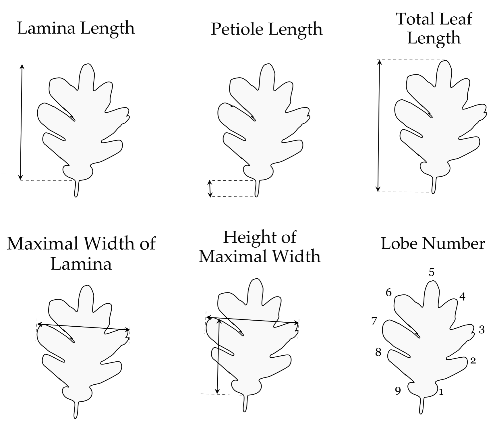
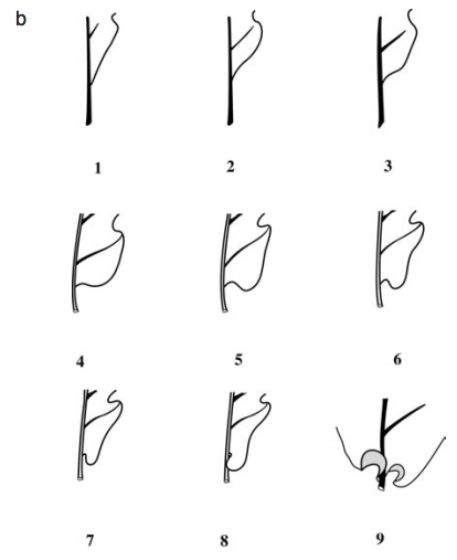
Figure 1. Morphological Traits description. A. Description of the leaf morphological traits in Quercus garryana and Q. robur. B. Scoring of the basal shape of the lamina (BS) of Quercus garryana and Q. robur. Figure 1B from Kremer et al., 2002.
Oak Leaves from their Native Range
I first wanted to create a dataset by measuring Quercus robur and Quercus garryana leaves from their native ranges so that these could be compared to the Portland Park and restoration area data (Figure 2). Because I could not travel to these areas to collect the information I needed, I utilized a digital herbarium database. Herbaria are compilations of physical specimens that people across the world have collected and preserved. These records document the flora and fauna that are present at a certain location during that moment in time. In recent decades, herbaria have been digitized so that people such as myself may use plant records from around the world in their research and everyday interests. I chose herbarium sheets from the iDigBio digital database, which features herbaria from across the world. This website contained 1.2 million herbaria records during the time I was gathering data for my research. I used iDigBio’s search engine in the same manner for both Quercus garryana and Quercus robur searches to control for possible differences in the types of herbarium sheets I came across.
After downloading images of oak leaves onto my laptop, I then used a program called ImageJ to measure the leaves for my physical traits of interest.
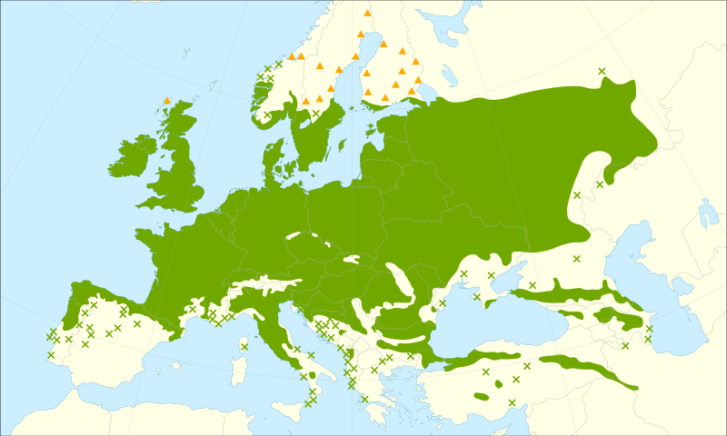
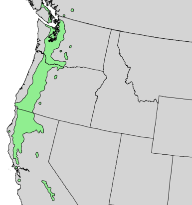
Figure 2. Q. robur and Q. garryana range maps A. Quercus robur range map. Triangles represent introduced populations.Wikipedia B. Quercus garryana range map. Wikipedia.
Oak Leaves in Portland
From November 3 to November 13, 2020, my thesis advisor, Keith Karoly, and I visited 13 sites in Portland Parks and natural areas and gathered leaves from 93 trees (Table 1). We utilized the Portland Parks and Recreation tree inventory map to find the trees by species within the parks. This database mapped trees by species onto the geography of Portland and was easily accessible. We printed maps of the parks and labeled each tree with a number. We used shears to clip small sections of leaves from each tree and placed them into a file folder after carefully labelling the tree number and folder section onto our map. I gained permission from the Portland Parks and Recreation to collect these samples via application for a research permit.
Table 1. Portland Parks This table lists parks where samples were collected, including the number of trees by proposed species.
Show code
Parks <- c("Argay City", "Lents", "Ed Benedict", "Farragut", "Laurelhurst", "Woodlawn", "Lair Hill", "Willamette", "West Moreland", "Powell Butte*", "Reed College Meadow*", "Oaks Bottom*", "Sellwood*")
Q.garryana <- c("3", "1","6", "5", "1", "1", "1", "5", "3", "10", "12", "2", "15")
Q.robur <- c("2", "5", "5", "5", "3", "1", "1", "5", "1", "-", "-", "-", "-")

park_names <- data.frame(Parks, Q.garryana, Q.robur)

park_names %>%
  gt()
| Parks | Q.garryana | Q.robur |
|---|---|---|
| Argay City | 3 | 2 |
| Lents | 1 | 5 |
| Ed Benedict | 6 | 5 |
| Farragut | 5 | 5 |
| Laurelhurst | 1 | 3 |
| Woodlawn | 1 | 1 |
| Lair Hill | 1 | 1 |
| Willamette | 5 | 5 |
| West Moreland | 3 | 1 |
| Powell Butte* | 10 | - |
| Reed College Meadow* | 12 | - |
| Oaks Bottom* | 2 | - |
| Sellwood* | 15 | - |
*Restoration areas.
These leaves were then taken back to the lab at Reed College and placed onto labeled sheets of paper and pressed using an herbarium plant press. These pressings were first dried at 50° C for one week and then stored until the samples could be properly photographed and affixed to herbarium sheets. To image the samples, I placed the leaves into a small studio called an Ortery Photosimile 200 - Desktop Product Photography Studio and then photographed the leaves using a Nikon 1 J5 mirrorless digital camera on a bench in the Karoly lab (Figure 3).
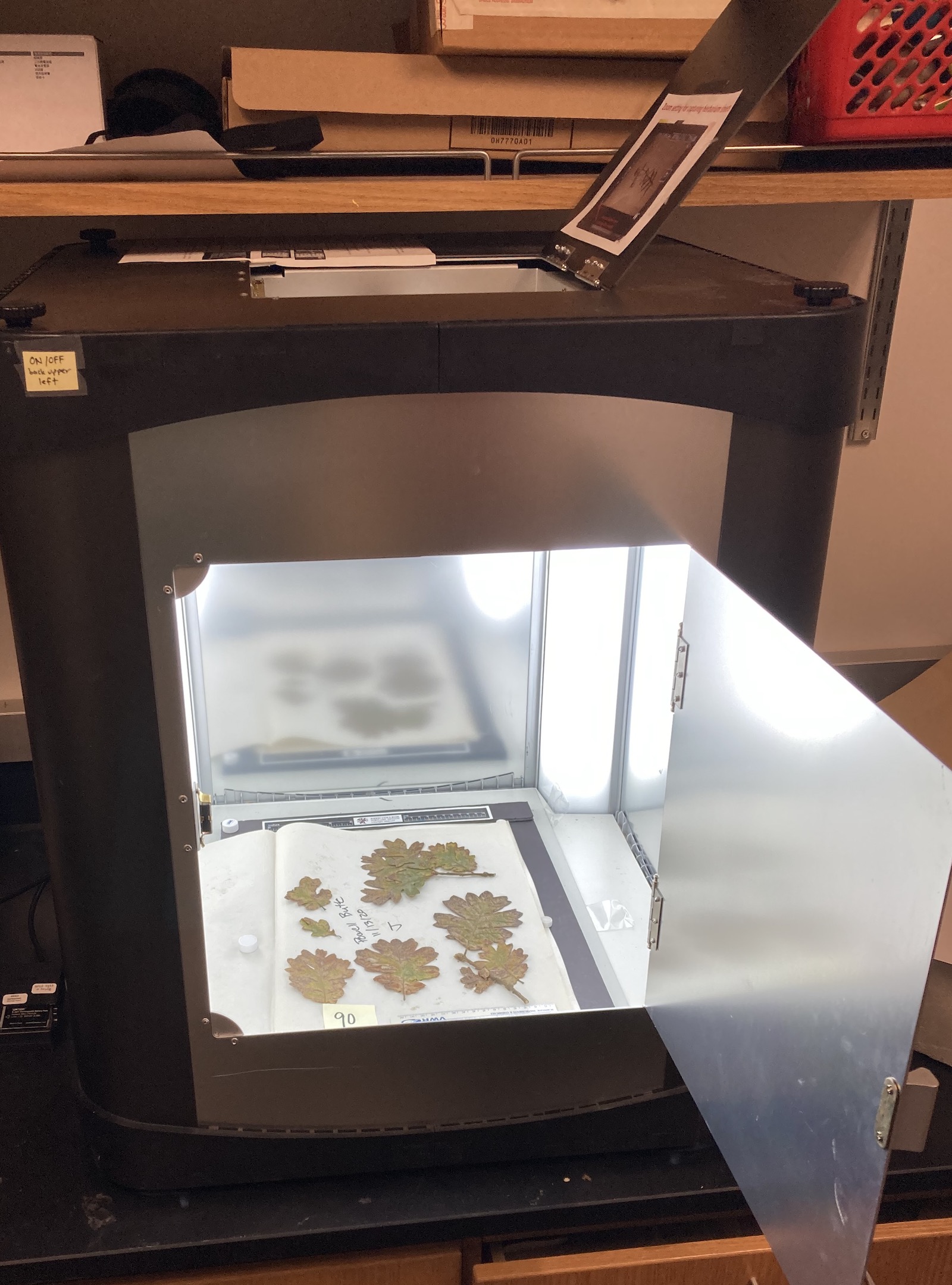
Figure 3. Photo of Imaging Set Up
K-means Clustering
The K-means cluster model divides the data into distinct k groups where the total variation within each cluster is as small as possible. This worked to create groups within the data that were most alike based on the present variables. Each time I wanted to know how well two variables predicted species, I would subset my data frame to only include the two variables of interest alongside their correct species.
From there, I plotted the proposed clusters mapped to color and the known species mapped to shape. If all of the shapes within each colored cluster were the same, then the variables on the x- and y- axes correctly predicted species.
I first computed k-means clusters on the native range dataset (Figure 4). This was necessary because I wanted to know how well this model could correctly identify a leaf’s species. We can see that only five of the 29 observations were incorrectly identified. This 83% rate of correct identifications influenced me to utilize this model on my Portland Park and restoration area data sets.
Show code
#LL and PL

landmarks1 <- landmarks %>%
  mutate(LLW = LL - HMW) %>%
  mutate(species = as.factor(species)) %>%
  select("species", "LL", "PL", "TLL", "MWL", "HMW", "LL_MWL", "LLW_MWL", "Petiole_percent", "LLW", "lobe_number")

set.seed(4)
diff_measures <- landmarks1

km_attempt10 = kmeans(diff_measures[, -1], centers = 2, nstart = 25)

diff_measures1 <- diff_measures %>%
  mutate(cluster = km_attempt10$cluster) %>%
  mutate(cluster = as.factor(cluster))

ggplot(data = diff_measures1, mapping = aes(y = LL, x = PL, color = cluster )) +
  geom_point(aes(shape = species)) +
  labs(x = "Petiole length (cm)", y = "Lamina length (cm)", title = "K means cluster for Oak Leaves in their Native Ranges")
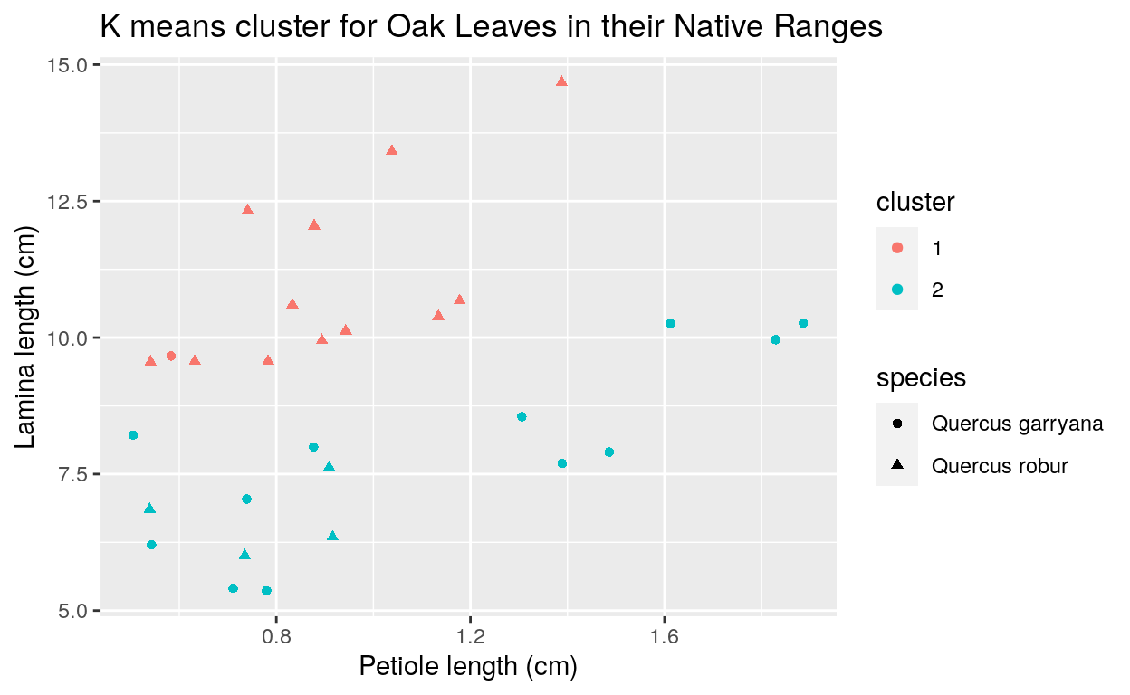
Figure 4. K-means cluster graph of lamina length and LLW/MWL for native range data.
I then used k-means clustering to see how well the model could identify species for the trees in Portland that the botanists held confidence concerning their species identification (Figure 5). Only 6 of the 34 observations were incorrectly identified. This is about 78% accuracy, which was not as impressive as the native range data, but still a rate that made it worth attempting species identification for the restoration areas.
Show code
  km_parks <- morphology %>%
  filter(image_id %in% c(19, 52, 25, 35, 59, 13, 64, 70, 50, 23, 79, 29, 34, 60, 17, 65, 67, 51)) %>%
  mutate(species = as.factor(species)) %>%
  mutate(LLW = LL - HMW) %>%
  drop_na(lobe_number) %>%
  mutate(lobe_number = as.numeric(lobe_number)) %>%
  select("species", "LL", "PL", "TLL", "MWL", "HMW", "LL_MWL", "LLW_MWL", "petiole_percent", "LLW", "lobe_number")

set.seed(4)
km_attempt_pdx5 = kmeans(km_parks[, -1], centers = 2, nstart = 25)

km_parks <- km_parks %>%
  mutate(cluster = km_attempt_pdx5$cluster) %>%
  mutate(cluster = as.factor(cluster))

ggplot(data = km_parks, mapping = aes(y = PL, x = petiole_percent, color = cluster )) +
  geom_point(aes(shape = species)) +
  scale_shape_manual(values = c(15, 17)) +
  labs(x = "Petiole percent", y = "Petiole length (cm)", title = "K means cluster for Portland Park Tree Leaves")
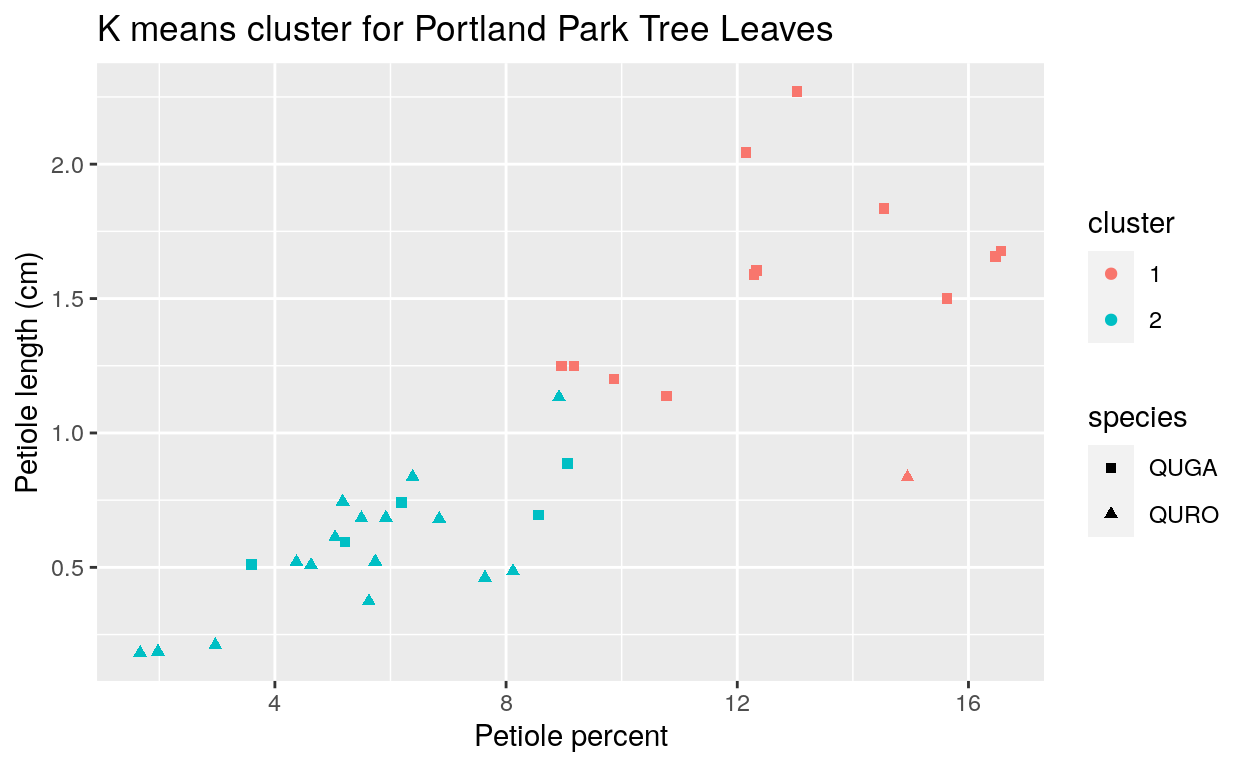
Figure 5. K-means cluster graph of petiole length and petiole percent for Portland Park data.
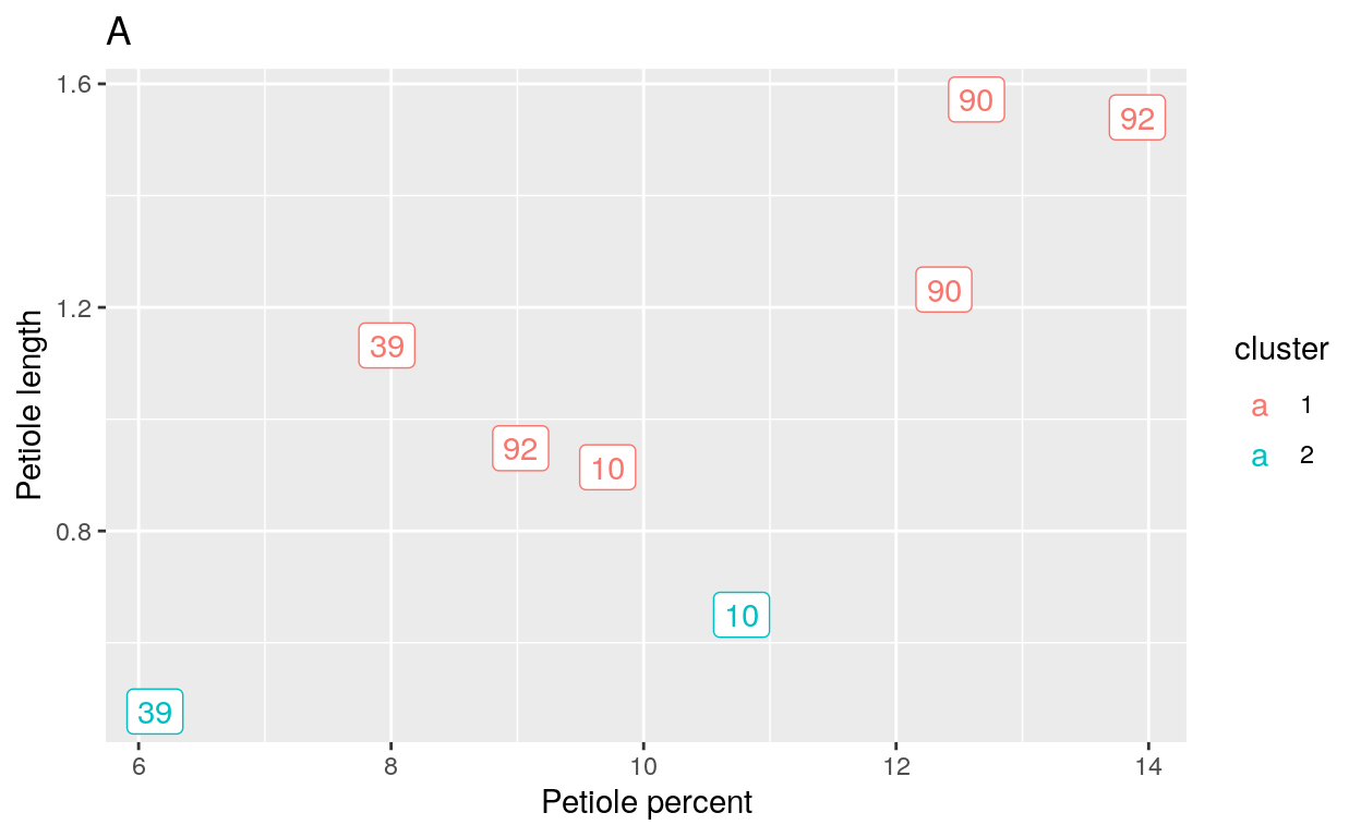
The final k-means cluster I made was with the hopes of identifying the species of the questionable trees in the restoration areas. I assigned these trees random labels and then plotted them in clusters of 2 and 3. The hope was that leaves of the same tree (ie their ID number) would group together and these means could be compared to the species from previous cluster plots.
When 2 clusters were placed on the model (Figure 6A), leaves from the same tree were placed into different clusters. The same was true when 3 clusters were placed as the parameter for the model (Figure 6B). This was problematic because the same tree in different clusters implied that the tree’s leaves were different species.
Show code
#k = 2
set.seed(4)
km_restore_areas <- morphology %>%
  filter(image_id %in% c(10, 39, 90, 92)) %>%
  mutate(LLW = LL - HMW) %>%
  drop_na(lobe_number) %>%
  mutate(lobe_number = as.numeric(lobe_number)) %>%
  mutate(species = as.factor(species)) %>%
  select("species", "LL", "PL", "TLL", "MWL", "HMW", "LL_MWL", "LLW_MWL", "petiole_percent", "LLW", "lobe_number")

#dropped two observations that have NAs

km_attempt_ra1 = kmeans(km_restore_areas[, -1], centers = 2, nstart = 25)

km_restore_areas <- km_restore_areas %>%
  mutate(cluster = km_attempt_ra1$cluster) %>%
  mutate(cluster = as.factor(cluster))

restoration_area <- morphology %>%
  filter(image_id %in% c(10, 39, 90, 92)) %>%
  mutate(LLW = LL - HMW) %>%
  drop_na(lobe_number) %>%
  mutate(cluster = km_attempt_ra1$cluster) %>%
  mutate(cluster = as.factor(cluster))

ggplot(data = km_restore_areas, mapping = aes(y = PL, x = petiole_percent, color = cluster)) +
  geom_point() +
  geom_label(data = restoration_area, aes(y = PL, x = petiole_percent, color = cluster, label = image_id), inherit.aes = FALSE) +
  labs(x = "Petiole percent", y = "Petiole length", title = "A")
Show code
# k = 3

set.seed(4)
km_attempt_ra2 = kmeans(km_restore_areas[, -1], centers = 3, nstart = 25)

km_restore_areas <- km_restore_areas %>%
  mutate(cluster = km_attempt_ra2$cluster) %>%
  mutate(cluster = as.factor(cluster))

restoration_area <- morphology %>%
  filter(image_id %in% c(10, 39, 90, 92)) %>%
  mutate(LLW = LL - HMW) %>%
  drop_na(lobe_number) %>%
  mutate(cluster = km_attempt_ra2$cluster) %>%
  mutate(cluster = as.factor(cluster))

ggplot(data = km_restore_areas, mapping = aes(y = PL, x = petiole_percent, color = cluster)) +
  geom_point() +
  geom_label(data = restoration_area, aes(y = PL, x = petiole_percent, color = cluster, label = image_id), inherit.aes = FALSE) +
  labs(x = "Petiole percent", y = "Petiole length", title = "B")
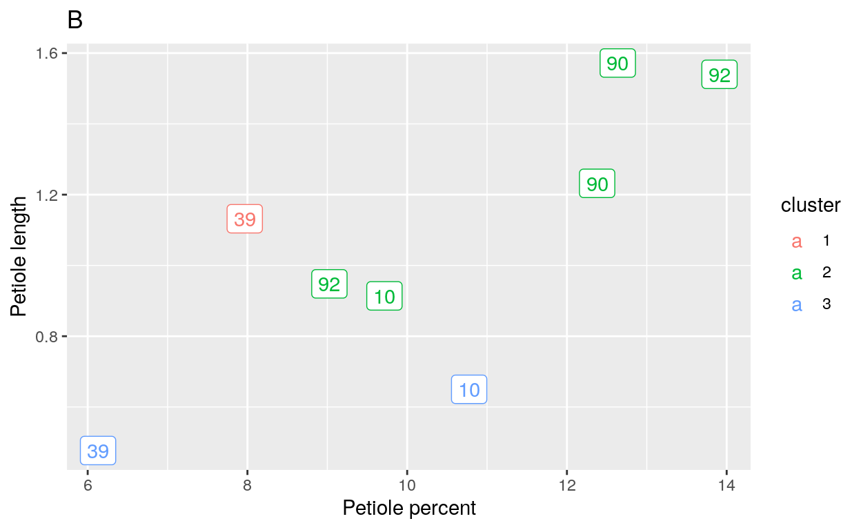
Figure 6 k-means Cluster Plots for Restoration Areas A. Cluster plot when k = 2. B. Cluster plot when k = 3. The numbers in the plots refer to the Image ID labels that belong to each tree.
My results suggested that though the k-means cluster model was the best analysis of the five models I considered, it was not conclusive in indicating the species of the trees in the Portland natural areas.
I do think that the identitiy of these trees could be found with more work! Future research on this question should involve statistical models that may more definitively classify the species of Portland natural and restoration area trees. Some suggestions for candidate models includes those mentioned in the literature such as, principle component analysis, canonical discriminant analysis, multiple correspondence analysis, factorial analysis of mixed data (Kremer et al., 2002; Rellstab et al., 2016; Tovar-sanchez and Oyama, 2004; Ekhvaia et al., 2018, Rushton, 1983. I also recommend including more leaves trees per site in the data set. Due to the amount of time I had available, I was not able to measure morphology in the lab for every tree I sampled from the field, so I am curious about how the expansion of the data set would influence the results.