The US Supreme Court: Unanimity and Unions

What kinds of Supreme Court decisions are unanimous? How does this change when the cases being decided are union cases?

Background

With recent high-profile coverage of unions (see American Factory, or the current key union case pending in the Supreme Court), we decided to take a look at decisions regarding union laws in the US Supreme Court (SCOTUS). This analysis was heavily supported by a comprehensive dataset on SCOTUS decisions, “The Supreme Court Database”, courtesy of law professor Harold Spaeth. This massive dataset spans the entire Court’s lifespan, from 1791 to 2020.

Two broad themes guided our analysis. First, we were interested in the split of the vote in SCOTUS decisions. Unanimous decisions in SCOTUS cases are not only the most frequent outcomes, but generally signal the clarity of the laws they provide guidance on. Therefore, when a unanimous decision is made, it indicates that the law being decided upon is very clear on how it is supposed to be interpreted.

Second, we were interested in alterations of precedent. SCOTUS is often reluctant to overturn precedent, and we expect that rates of precedent alteration are generally low. More importantly, alterations of precedent indicate either that the deciding court thinks the previous court made a mistake in its interpretation of the law, or that shifts in political or cultural decisions lend weight to the argument that other legal principles outweigh the principle of respecting precedent.

Data Wrangling

First we renamed the the data sets into the names “cases” and “justices”.

Show code

cases_ <- SCDB_2020_01_caseCentered_LegalProvision
justices_ <- SCDB_2020_01_justiceCentered_LegalProvision

We then did some light cleaning on the columns: we changed the class and format of the variable “dateDecision” to be a date class.

Show code

data$dateDecision <- as.Date(data$dateDecision, format = "%Y-%m-%d")

In addition, we noticed that the datasets contained many duplicate observations and thus filtered to remove these duplicates.

Show code

cases <- cases %>% filter(lawType == 3) # Select federal law types and remove duplicate cases
cases <- cases[!duplicated(cases$caseId),]
cases <- cases %>% select(-c("lawType"))

justices <- justices %>% filter(lawType == 3) # Select federal law types and remove duplicate cases
justices <- justices[!duplicated(justices$caseId),] # Bug: need to do some join stuff to get justices (they arent dupes)
justices <- justices %>% select(-c("lawType"))

In order to make the themes of the data more clear, we performed a join and added the variable “issue_topic” which further explains the variable “issue”.

Show code

  issue_key <- read_csv(file = "issue_key.csv")
  colnames(issue_key) <- c("issueArea","Issue")
  issue_key$Issue <- as.factor(issue_key$Issue)
  issue_key$issueArea <- as.factor(issue_key$issueArea)
  cases <- right_join(cases, issue_key, by = "issueArea")

We then selected variables that we were interested in.

Show code

cases <- cases_ %>% 
  select(caseId, caseName,
         dateDecision, decisionType, decisionDirection, 
         majOpinWriter, majVotes, minVotes, 
         precedentAlteration, lawType, issue, issueArea,
         caseSourceState)

justices <- justices_ %>% 
  select(caseId, caseName,
         justice, justiceName, direction, opinion, vote,
         dateDecision, decisionType, decisionDirection, 
         majOpinWriter, majVotes, minVotes, 
         precedentAlteration, lawType, issue, issueArea,
         caseSourceState)

We also exported the datasets so that they could be reproduced for future study.

Show code

if(write){
  write.csv(cases, "data/cases.csv", row.names = F)
  write.csv(justices, "data/justices.csv", row.names = F)
}

Finally, we used mutate to do some computations in order to make further claims with our data.

Show code

props <- right_join(issue_counts, class_counts, "Issue") %>% mutate(prop = 100 * n/count)

Guiding Questions

For SCOTUS cases in general and SCOTUS union cases:

• How unanimous are the decisions made?

• What proportion of cases are decided in the liberal, neutral or conservative direction?

• How does unanimity differ based on decision direction?

• How does precedent alteration differ based on decision direction?

A Unanimity Statistic

One statistic that is observed is the unanimity of Supreme Court decisions. While the raw number of ‘majority’ votes is a good indicator, an ever-changing problem of number of justices poses a problem of shifting interpretations. To address this problem, we create a normalized value called the unanimity score that is independent of the number of justices.

We first take the ratio of the number of minority votes to that of the majority votes, then take one minus this ratio, as follows:

\[ u= 1−\frac{minority}{majority} \]

This latter step ensures that a score of 1 corresponds to unanimity, as opposed to no majority. A greater score implies a greater majority.

The table below displays the scores, the names of the classes, and how many justices would be in the majority if the case was heard by nine justices:

Show code

table_ %>%
  gt() %>%
  tab_header(title = "Unanimity") %>%
  cols_label("unanimity" = "Unanimity Score", 
                     "unanimity_class" = "Class",
             "maj" = "Majority Vote on a Nine-Justice Court") %>%
  tab_source_note(source_note = "Ties can only exist in Supreme Courts where there are an even number of justices.  A Unanimity Score of 0 indicates a vote that resulted in a tie/had no majority.") %>%
  data_color(
columns = vars("unanimity_class"),
colors = scales::col_factor(as.character(paletteer::paletteer_d("RColorBrewer::RdYlBu")),
                             domain = c("No Majority", 
                                        "Slight Majority", 
                                        "Moderate Majority", 
                                        "Large Majority", "
                                        Unanimous"),
                            ordered = TRUE))

Unanimity
Unanimity Score	Class	Majority Vote on a Nine-Justice Court
0.200	Slight Majority	5
0.500	Moderate Majority	6
0.714	Large Majority	7
0.875	Large Majority	8
1.000	Unanimous	9
Ties can only exist in Supreme Courts where there are an even number of justices. A Unanimity Score of 0 indicates a vote that resulted in a tie/had no majority.

The Investigation

General Supreme Court Cases

Show code

unanimity_prop_barplot(cases, union = F)

Show code

conditional_table(cases, unanimity, Issue) %>%
  gt() %>%
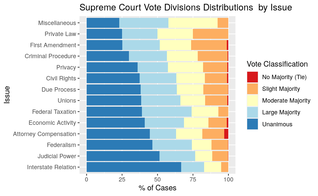
  tab_header(title = "Supreme Court Vote Divisions Distributions by Issue") %>%
  cols_label("Issue" = "Issue", 
                     "median" = "Median",
             "mean" = "Mean",
             "sd" = "Standard Deviation",
             "sample_size" = "Sample Size")

Supreme Court Vote Divisions Distributions by Issue
Issue	Median	Mean	Standard Deviation	Sample Size
Interstate Relation	1.0000000	0.8699134	0.2318574	99
Judicial Power	1.0000000	0.7945279	0.2747652	1237
Federal Taxation	0.8750000	0.7757607	0.2469457	313
Federalism	0.8750000	0.7659495	0.2787929	410
Economic Activity	0.8571429	0.7360733	0.2915363	1761
Unions	0.8571429	0.7199050	0.2985419	361
Civil Rights	0.7142857	0.7052921	0.3005662	1464
Attorney Compensation	0.8571429	0.7049468	0.3252881	103
Due Process	0.7142857	0.7012655	0.3041449	349
Privacy	0.7142857	0.6813085	0.3073297	117
Miscellaneous	0.7142857	0.6709707	0.2542570	26
Criminal Procedure	0.7142857	0.6515606	0.3054490	2039
Private Law	0.6875000	0.6437500	0.3642201	4
First Amendment	0.6666667	0.6169604	0.3130198	685

This pattern by issue generally conforms with our expectations: the more contentious issues tend to have lower proportions of unanimous decisions, and vice versa. Interestingly for us, union cases actually sit midway between the two poles!

Show code

props %>%
    filter(!is.na(decisionDirection)) %>%
    ggplot(aes(x = decisionDirection, y = prop, fill = unanimity_class)) +
    geom_bar(stat = "identity") +  
    scale_x_discrete(guide = guide_axis(n.dodge = 1)) +
    scale_fill_brewer(type = "seq", palette = "RdYlBu")+
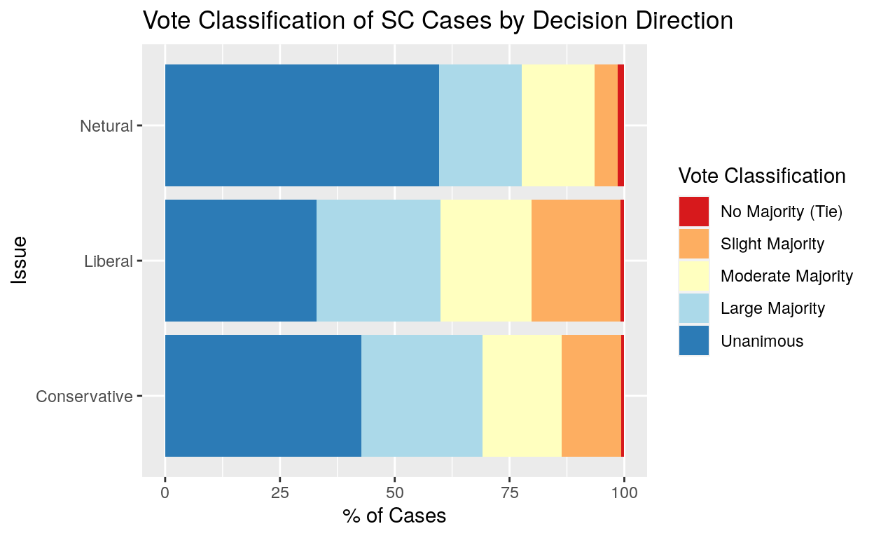
    labs(fill = "Vote Classification",title = "Vote Classification of SC Cases by Decision Direction", x = "Issue", y = "% of Cases") +
    coord_flip()

Show code

conditional_table(cases, unanimity, decisionDirection) %>%
  gt() %>%
  tab_header(title = "Unanimity Scores by Decision Direction") %>%
  cols_label("decisionDirection" = "Decision Direction", 
                     "median" = "Median",
             "mean" = "Mean",
             "sd" = "Standard Deviation",
             "sample_size" = "Sample Size")

Unanimity Scores by Decision Direction
Decision Direction	Median	Mean	Standard Deviation	Sample Size
Netural	1.0000000	0.8293165	0.2620927	139
Conservative	0.8750000	0.7432293	0.2897464	4530
Liberal	0.7142857	0.6747137	0.3060840	4299

It is generally difficult to pin down whether a decision is liberal or conservative for specific cases. The codebook notes that the dataset creators defined a decision as liberal if it corresponded to an advancement of liberal causes, such as “pro-union”, “pro-female in abortion”, “pro-federal power” and so on, with conservative defined as the exact opposite.

The proportion plot shows the breakdown of discrete vote classifications by decision direction, while the table provides summary statistics of the continuous unanimity scores. The split by vote classes show that a greater proportion of conservative decisions are unanimous than liberal decisions - nearly 10% more! We also find that this pattern is reversed in votes involving slight majorities, whereby 10% more of liberal decisions involve slight majorities. Finally, we see that most SCOTUS decisions are based on large majorities or unanimous votes, as opposed to slight majorities and tie votes.

The table indicates that that liberal decisions tend to have a lower unanimity score than conservative and neutral decisions (lower median and mean). It further shows in the sample size column that a minuscule number of decisions are classified as neutral, and the vast majority are either liberal or conservative.

Show code

cases %>%
  group_by(decisionDirection) %>%
  summarize(perc_alterations = 100 * mean(precedentAlteration)) %>%
  gt() %>%
  tab_header(title = "Decision Direction vs. Precedent Alterations") %>%
  cols_label("decisionDirection" = "Decision Direction", 
                     "perc_alterations" = "Rate of Precedent Alterations")

Decision Direction vs. Precedent Alterations
Decision Direction	Rate of Precedent Alterations
Conservative	2.428256
Liberal	1.744592
Netural	0.000000

Unsurprisingly, this table shows that the absolute rates of precedent alterations for general SCOTUS decisions are low for both kinds of decision direction. It also shows that the rate of precedent alteration for conservative decisions is slightly greater than the rate for liberal decisions.

Union Cases

Show code

props %>%
    filter(!is.na(decisionDirection)) %>%
    ggplot(aes(x = decisionDirection, y = prop, fill = unanimity_class)) +
    geom_bar(stat = "identity") +  
    scale_x_discrete(guide = guide_axis(n.dodge = 1)) +
    scale_fill_brewer(type = "seq", palette = "RdYlBu")+
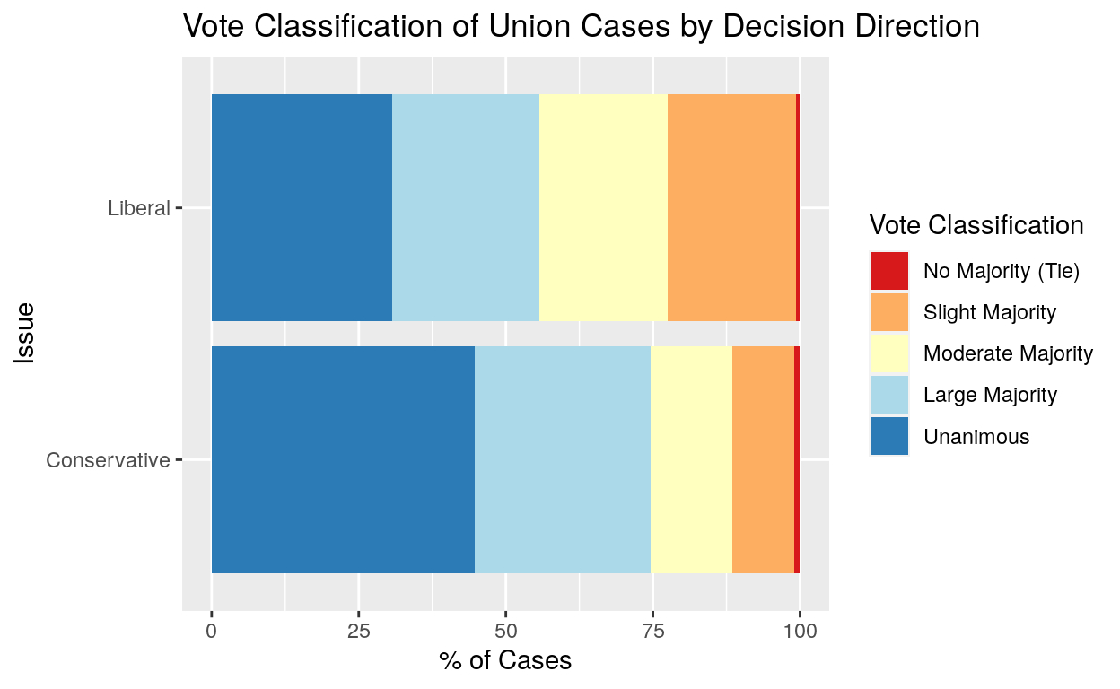
    labs(fill = "Vote Classification",title = "Vote Classification of Union Cases by Decision Direction", x = "Issue", y = "% of Cases") +
    coord_flip()

Show code

conditional_table(union_cases, unanimity, decisionDirection) %>%
  gt() %>%
  tab_header(title = "Unanimity Scores of Union Cases by Decision Direction") %>%
  cols_label("decisionDirection" = "Decision Direction", 
                     "median" = "Median",
             "mean" = "Mean",
             "sd" = "Standard Deviation",
             "sample_size" = "Sample Size")

Unanimity Scores of Union Cases by Decision Direction
Decision Direction	Median	Mean	Standard Deviation	Sample Size
Conservative	0.8750000	0.7679578	0.2790695	201
Liberal	0.7142857	0.6595387	0.3118487	160

The proportion plot and table shown above mirror those displayed for general SCOTUS decisions. And indeed, the pattern of vote classes among these union cases is very similar to the pattern among general SCOTUS cases: a greater proportion of conservative decisions are unanimous than liberal decisions, and the pattern is reversed in decisions involving slight majorities.

The table reinforces the conclusions drawn above, and also demonstrates that more SCOTUS union decisions are conservative than liberal.

Show code

union_cases %>%
  group_by(decisionDirection) %>%
  summarize(perc_alterations = 100 * mean(precedentAlteration)) %>%
  gt() %>%
  tab_header(title = "Precedent Alterations") %>%
  cols_label("decisionDirection" = "Decision Direction", 
                     "perc_alterations" = "Rate of Precedent Alterations")

Precedent Alterations
Decision Direction	Rate of Precedent Alterations
Conservative	0.4975124
Liberal	2.5000000

Here, as in the general SCOTUS decision analysis, we find that the absolute rates of precedent alterations are low for both kinds of decision direction. However, the rate of precedent alteration for liberal decisions is more than five times that of conservative decisions!

Conclusions and Implications:

Here is the summary of our conclusions, and the implications of those conclusions.

• First, the patterns of unanimity across general SCOTUS decisions are roughly similar to that of union SCOTUS decisions - across both, a plurality of decisions are unanimous, and a majority of the decisions involve unanimous or large majority votes.
  • This makes sense, given that union cases sit in the middle in terms of unanimous decisions (see the first figure). It also aligns with our expectations about unanimity in SCOTUS decisions - namely, that a plurality of SCOTUS decisions are unanimous.
• Second, across decision direction, more conservative decisions are classed as unanimous/large majority than liberal decisions, and the median and mean unanimity scores across both show the same pattern.
  • The implication here is that, on the judicial level, either (1) fewer justices agree when the decision is liberal or (2) more justices agree when the decision is conservative. Alternatively, on the level of lawmaking, we could argue that our hypothesis is true: the “law as intended/interpreted” for these cases tends to lean conservative.
• Third, across both general and union SCOTUS cases, more decisions are decided in the conservative direction than the liberal direction.
  • This implies, as we might expect, that SCOTUS decisions generally lean conservative.
• Finally, precedent alteration occurs more in conservative decisions than in liberal decisions in general SCOTUS cases, but the pattern is reversed for union SCOTUS cases.
  • This may imply that union laws are generally written to be anti-union. Since more union decisions that are liberal alter precedent, this can mean that the court’s previous interpretations of those laws (ie. precedent) lean conservative. However, as we stated in our introduction, this may also simply mean that the deciding courts were engaged in conservative judicial activism.